Section author: Danielle J. Navarro and David R. Foxcroft
The independent samples t-test (Welch test)
The biggest problem with using the Student test in practice is the third
assumption listed in the previous section. It assumes that both groups have
the same standard deviation. This is rarely true in real life. If two samples
don’t have the same means, why should we expect them to have the same standard
deviation? There’s really no reason to expect this assumption to be true.
We’ll talk a little bit about how you can check this assumption later on
because it does crop up in a few different places, not just the t-test. But
right now I’ll talk about a different form of the t-test (Welch, 1947) that does not rely on this assumption. A graphical illustration
of what the Welch t test assumes about the data is shown in
Fig. 92, to provide a contrast with the Student test version
in Fig. 90. I’ll admit it’s a bit odd to talk about the cure
before talking about the diagnosis, but as it happens the Welch's test can
be specified as one of the Independent Samples T-Test options in jamovi,
so this is probably the best place to discuss it.

Fig. 92 Graphical illustration of the null and alternative hypotheses assumed by the Welch t-test. Like the Student t-test for Independent Samples (Fig. 90) we assume that both samples are drawn from a normally-distributed population; but the alternative hypothesis no longer requires the two populations to have equal variance.
The Welch test is very similar to the Student test. For example, the t-statistic that we use in the Welch test is calculated in much the same way as it is for the Student test. That is, we take the difference between the sample means and then divide it by some estimate of the standard error of that difference:
The main difference is that the standard error calculations are different. If the two populations have different standard deviations, then it’s a complete nonsense to try to calculate a pooled standard deviation estimate, because you’re averaging apples and oranges.[1]
But you can still estimate the standard error of the difference between sample means, it just ends up looking different
The reason why it’s calculated this way is beyond the scope of this book. What matters for our purposes is that the t-statistic that comes out of the Welch t-test is actually somewhat different to the one that comes from the Student t-test.
The second difference between Welch and Student is that the degrees of freedom are calculated in a very different way. In the Welch test, the “degrees of freedom” doesn’t have to be a whole number any more, and it doesn’t correspond all that closely to the “number of data points minus the number of constraints” heuristic that I’ve been using up to this point.
The degrees of freedom are, in fact
which is all pretty straightforward and obvious, right? Well, perhaps not. It doesn’t really matter for our purposes. What matters is that you’ll see that the “df” value that pops out of a Welch test tends to be a little bit smaller than the one used for the Student test, and it doesn’t have to be a whole number.
Doing the Welch test in jamovi
If you tick the check box for the Welch's test in the analysis we did
above, then this is what it gives you Fig. 93:
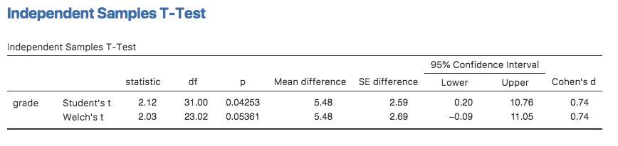
Fig. 93 Results showing the Welch test alongside the default Student’s t-test in jamovi
The interpretation of this output should be fairly obvious. You read the output for the Welch’s test in the same way that you would for the Student’s test. You’ve got your descriptive statistics, the test results and some other information. So that’s all pretty easy.
Except, except… our result isn’t significant anymore. When we ran the Student test we did get a significant effect, but the Welch test on the same data set is not (t(23.02) = 2.03, p = 0.054). What does this mean? Should we panic? Is the sky burning? Probably not. The fact that one test is significant and the other isn’t doesn’t itself mean very much, especially since I kind of rigged the data so that this would happen. As a general rule, it’s not a good idea to go out of your way to try to interpret or explain the difference between a p-value of 0.049 and a p-value of 0.051. If this sort of thing happens in real life, the difference in these p-values is almost certainly due to chance. What does matter is that you take a little bit of care in thinking about what test you use. The Student test and the Welch test have different strengths and weaknesses. If the two populations really do have equal variances, then the Student test is slightly more powerful (lower Type II error rate) than the Welch test. However, if they don’t have the same variances, then the assumptions of the Student test are violated and you may not be able to trust it; you might end up with a higher Type I error rate. So it’s a trade off. However, in real life I tend to prefer the Welch test, because almost no-one actually believes that the population variances are identical.
Assumptions of the test
The assumptions of the Welch test are very similar to those made by the Student t-test (see Assumptions of the Student *t*-test), except that the Welch test does not assume homogeneity of variance. This leaves only the assumption of normality and the assumption of independence. The specifics of these assumptions are the same for the Welch test as for the Student test.
| [1] | Well, I guess you can average apples and oranges, and what you end up with is a delicious fruit smoothie. But no one really thinks that a fruit smoothie is a very good way to describe the original fruits, do they? |