Forfatter av avsnitt: Danielle J. Navarro and David R. Foxcroft

z-testen med ett utvalg

In this section I will describe one of the most useless tests in all of statistics: the z-test. Seriously – this test is almost never used in real life. Its only real purpose is that, when teaching statistics, it is a very convenient stepping stone along the way towards the t-test, which is probably the most (over)used tool in all statistics.

Inferensproblemet som testen tar for seg

To introduce the idea behind the z-test, let us use a simple example. A friend of mine, Dr Zeppo, grades his introductory statistics class on a curve. Let us suppose that the average grade in his class is 67.5, and the standard deviation is 9.5. Of his many hundreds of students, it turns out that 20 of them also take psychology classes. Out of curiosity, I find myself wondering if the psychology students tend to get the same grades as everyone else (i.e., the mean of 67.5) or do they tend to score higher or lower? He emails me the zeppo data set, which I use to look at the grades of those students, in the jamovi spreadsheet view,

50 60 60 64 66 66 67 69 70 74 76 76 77 79 79 79 81 82 82 89

og beregner deretter gjennomsnittet i Exploration → Descriptives. Gjennomsnittsverdien er 72,3.

It appears as if the psychology students were scoring a bit higher than normal. That sample mean of X̄ = 72.3 is a fair bit higher than the hypothesised population mean of µ = 67.5 but, on the other hand, a sample size of N = 20 is not that big. Maybe it is pure chance.

To answer the question, it helps to be able to write down what it is that I think I know. Firstly, I know that the sample mean is X̄ = 72.3. If I am willing to assume that the psychology students have the same standard deviation as the rest of the class then I can say that the population standard deviation is σ = 9.5. I will also assume that since Dr Zeppo is grading to a curve, the psychology student grades are normally distributed.

Next, it helps to be clear about what I want to learn from the data. In this case my research hypothesis relates to the population mean µ for the psychology student grades, which is unknown. Specifically, I want to know if µ = 67.5 or not. Given that this is what I know, can we devise a hypothesis test to solve our problem? The data, along with the hypothesised distribution from which they are thought to arise, are shown in Fig. 97. Not entirely obvious what the right answer is, is it? For this, we are going to need some statistics.

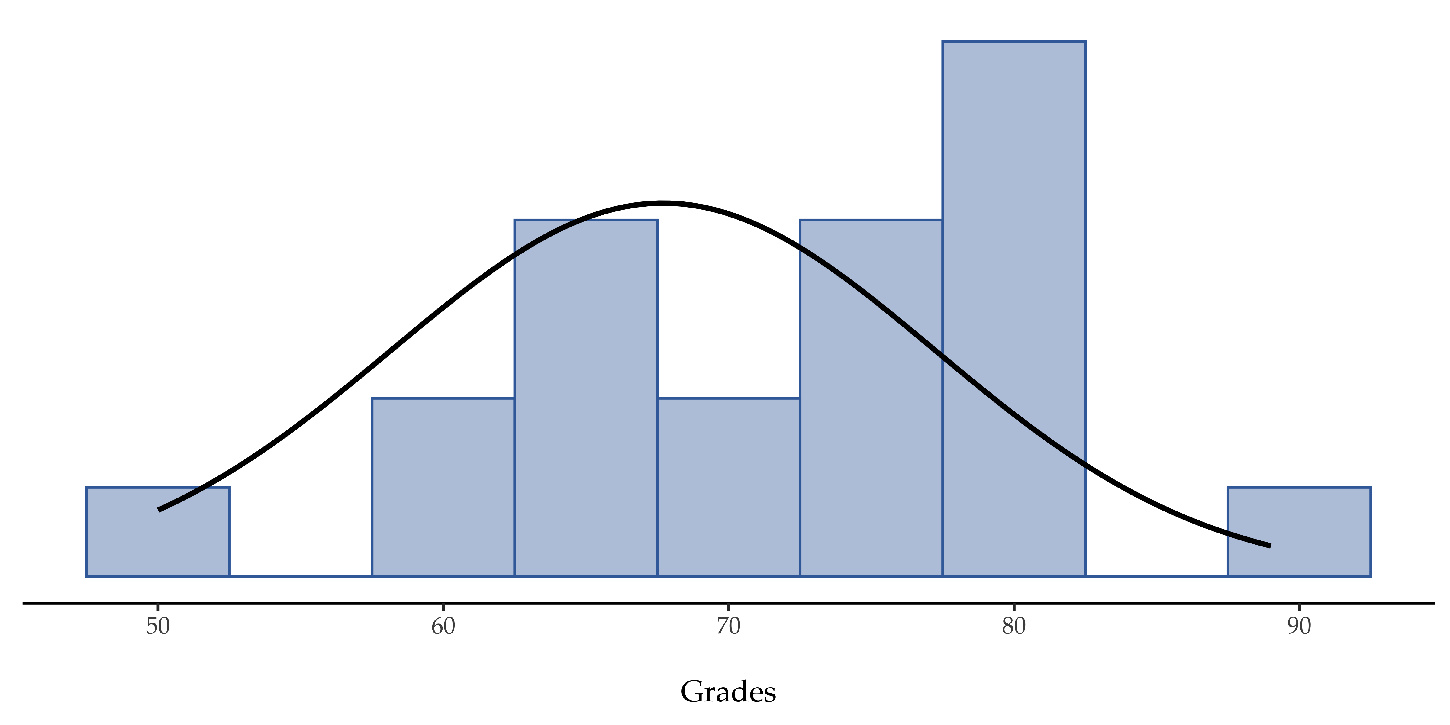
Fig. 97 Den teoretiske fordelingen (heltrukken linje) som psykologistudentenes karakterer (søyler) antas å ha blitt generert fra.

Gjennomføring av hypotesetesten

The first step in constructing a hypothesis test is to be clear about what the null and alternative hypotheses are. This is not too hard to do. Our null hypothesis, H₀, is that the true population mean µ for psychology student grades is 67.5%, and our alternative hypothesis is that the population mean is not 67.5%. If we write this in mathematical notation, these hypotheses become:

H₀: µ = 67.5

H₁: µ ≠ 67.5

though to be honest this notation does not add much to our understanding of the problem, it is just a compact way of writing down what we are trying to learn from the data. The null hypotheses H₀ and the alternative hypothesis H₁ for our test are both illustrated in Fig. 98. In addition to providing us with these hypotheses, the scenario outlined above provides us with a fair amount of background knowledge that might be useful. Specifically, there are two special pieces of information that we can add:

1. Psykologikarakterene er normalfordelte.

2. Det sanne standardavviket for disse poengene σ er kjent for å være 9,5.

For the moment, we will act as if these are absolutely trustworthy facts. In real life, this kind of absolutely trustworthy background knowledge does not exist, and so if we want to rely on these facts we will just have to make the assumption that these things are true. However, since these assumptions may or may not be warranted, we might need to check them. For now though, we will keep things simple.

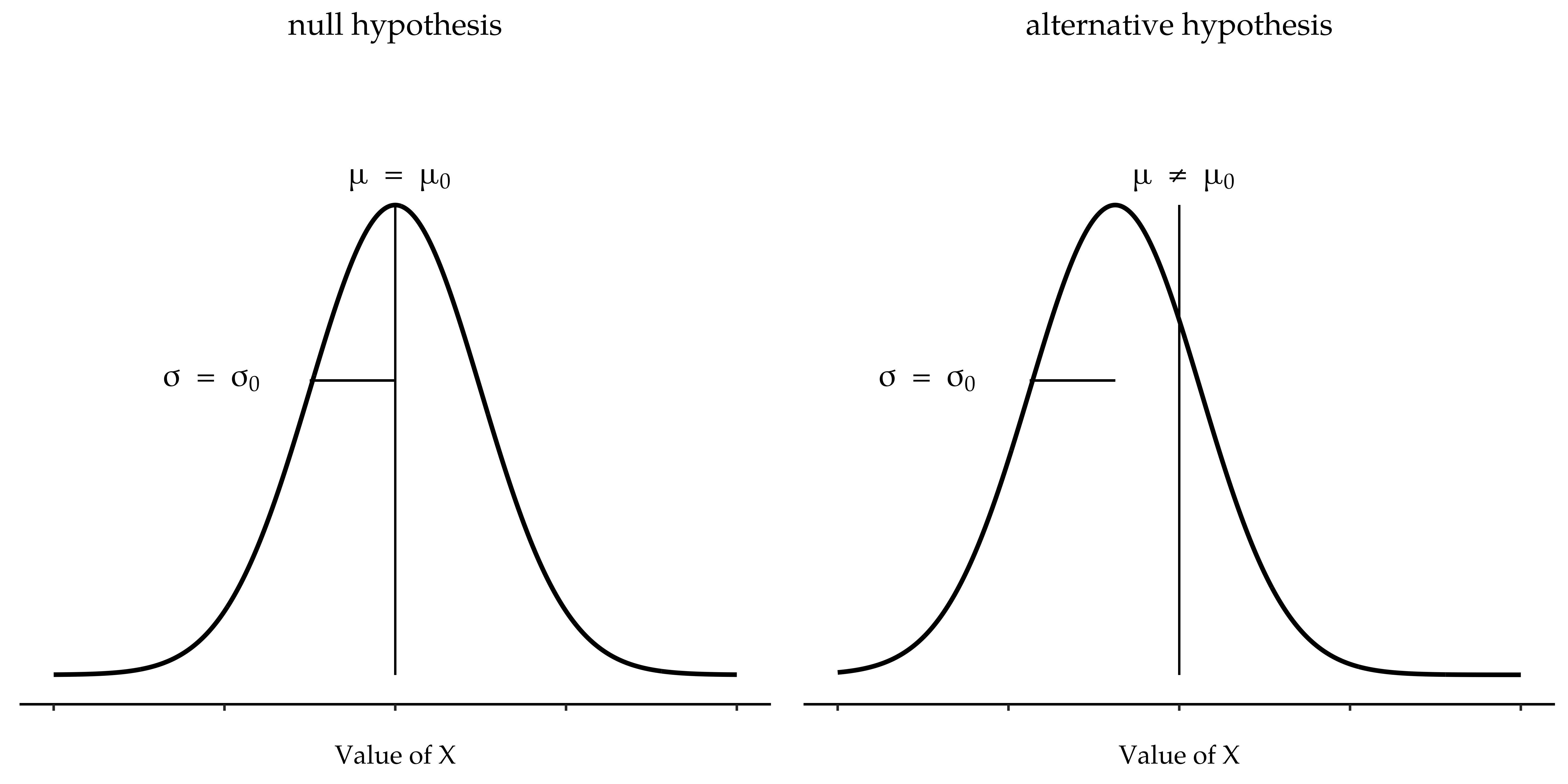
Fig. 98 Grafisk illustrasjon av nullhypotesen og alternativhypotesen i z-testen for ett utvalg (den tosidige versjonen). Nullhypotesen og alternativhypotesen forutsetter begge at populasjonen er normalfordelt, og i tillegg forutsettes det at populasjonens standardavvik er kjent (fastsatt til en verdi σ₀). Nullhypotesen (til venstre) er at populasjonsgjennomsnittet μ er lik en spesifisert verdi μ₀. Alternativhypotesen er at populasjonsgjennomsnittet avviker fra denne verdien, μ ≠ μ₀.

The next step is to figure out what would be a good choice for a diagnostic test statistic, something that would help us discriminate between H₀ and H₁. Given that the hypotheses all refer to the population mean µ, you would feel pretty confident that the sample mean X̄ would be a pretty useful place to start. What we could do is look at the difference between the sample mean X̄ and the value that the null hypothesis predicts for the population mean. In our example that would mean we calculate X̄ - 67.5. More generally, if we let µ₀ refer to the value that the null hypothesis claims is our population mean, then we would want to calculate:

X̄ - µ₀

If this quantity equals or is very close to 0, things are looking good for the null hypothesis. If this quantity is a long way away from 0, then it is looking less likely that the null hypothesis is worth retaining. But how far away from zero should it be for us to reject H₀?

To figure that out we need to be a bit more sneaky, and we will need to rely on those two pieces of background knowledge that I wrote down previously; namely that the raw data are normally distributed and that we know the value of the population standard deviation σ. If the null hypothesis is actually true, and the true mean is µ₀, then these facts together mean that we know the complete population distribution of the data: a normal distribution with mean µ₀ and standard deviation σ. Adopting the notation from section Normalfordelingen, a statistician might write this as:

X ~ Normal(µ₀, σ²)

Okay, if that is true, then what can we say about the distribution of X̄? Well, as we discussed earlier (see The central limit theorem), the sampling distribution of the mean X̄ is also normal, and has mean µ. But the standard deviation of this sampling distribution SE(X̄), which is called the standard error of the mean, is:

\[SE(X̄) = \frac{\sigma}{\sqrt{N}}\]

Med andre ord, hvis nullhypotesen er sann, kan utvalgsfordelingen av gjennomsnittet skrives som følger:

X̄ ~ Normal(µ₀, SE(X̄))

Now comes the trick. What we can do is convert the sample mean X̄ into a standard score. This is conventionally written as z, but for now I am going to refer to it as z_X̄. The reason for using this expanded notation is to help you remember that we are calculating a standardised version of a sample mean, not a standardised version of a single observation, which is what a z-score usually refers to. When we do so the z-score for our sample mean is:

\[z_{\bar{X}} = \frac{\bar{X} - \mu_0}{SE(X̄)}\]

eller, tilsvarende:

\[z_{\bar{X}} = \frac{\bar{X} - \mu_0}{\sigma / \sqrt{N}}\]

Denne z-scoren er teststatistikken vår. Det fine med å bruke denne som teststatistikk er at den, i likhet med alle z-skårer, har en standard normalfordeling:

z_*X̄* ~ Normal(0, 1)

(again, see section z-verdier if you have forgotten why this is true). In other words, regardless of what scale the original data are on, the z-statistic itself always has the same interpretation: it is equal to the number of standard errors that separate the observed sample mean X̄ from the population mean µ₀ predicted by the null hypothesis. Better yet, regardless of what the population parameters for the raw scores actually are, the 5% critical regions for the z-test are always the same, as illustrated in Fig. 99. And what this meant, way back in the days where people did all their statistics by hand, is that someone could publish a table like this:

ønsket α-nivå	tosidig test	ensidig test
0.1	1.644854	1.281552
0.05	1.959964	1.644854
0.01	2.575829	2.326348
0.001	3.290527	3.090232

Det betydde i sin tur at forskerne kunne regne ut z-statistikken for hånd og deretter slå opp den kritiske verdien i en lærebok.

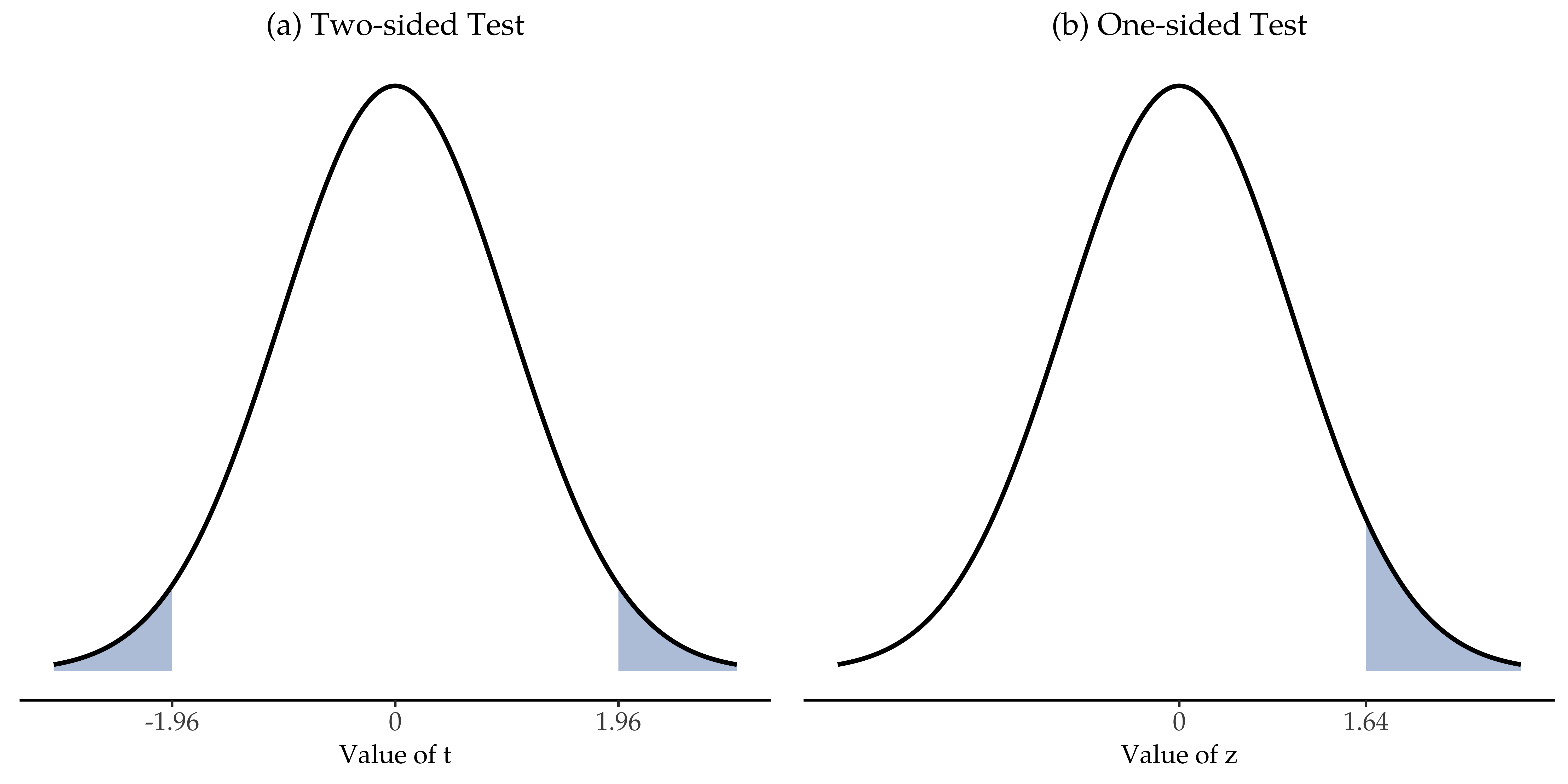
Fig. 99 Avvisningsregioner for den tosidige z-testen (venstre panel) og den ensidige z-testen (høyre panel)

Et bearbeidet eksempel, for hånd

Now, as I mentioned earlier, the z-test is almost never used in practice. It is so rarely used in real life that the basic installation of jamovi does not have a built-in function for it. However, the test is so incredibly simple that it is really easy to do one manually. Let us go back to the zeppo data set. The first thing I need to do is calculate the sample mean for the grades variable, which I have already done (72.3). We already have the known population standard deviation (σ = 9.5), and the value of the population mean that the null hypothesis specifies (µ₀ = 67.5), and we know the sample size (N = 20).

Next, let us calculate the (true) standard error of the mean (easily done with a calculator):

sem.true = sd.true / sqrt(N)
         = 9.5 / sqrt(20)
         = 2.124265

Til slutt beregner vi z-poengsummen vår:

z.score  = (sample.mean - mu.null) / sem.true
         = (72.3 - 67.5) / 2.124265
         = 2.259606

At this point, we would traditionally look up the value 2.26 in our table of critical values. Our original hypothesis was two-sided (we did not really have any theory about whether psych students would be better or worse at statistics than other students) so our hypothesis test is two-sided (or two-tailed) also. Looking at the little table that I showed earlier, we can see that 2.26 is bigger than the critical value of 1.96 that would be required to be significant at α = 0.05, but smaller than the value of 2.58 that would be required to be significant at a level of α = 0.01. Therefore, we can conclude that we have a significant effect, which we might write up by saying something like this:

Med en gjennomsnittskarakter på 72,3 i utvalget av psykologistudenter, og forutsatt et standardavvik i populasjonen på 9,5, kan vi konkludere med at psykologistudentene har signifikant forskjellige statistikkpoengsummer enn gjennomsnittet i klassen (z = 2,26, N = 20, p < 0,05).

Forutsetninger for z-testen

As I have said before, all statistical tests make assumptions. Some tests make reasonable assumptions, while other tests do not. The test I have just described, the one sample z-test, makes three basic assumptions. These are:

• Normality. As usually described, the z-test assumes that the true population distribution is normal.[1] This is often a pretty reasonable assumption, and it is also an assumption that we can check if we feel worried about it (see section Sjekk forutsetningen om normalfordeling for en stikkprøve).

• Independence. The second assumption of the test is that the observations in your data set are not correlated with each other, or related to each other in some funny way. This is not as easy to check statistically, it relies a bit on good experimental design. An obvious (and stupid) example of something that violates this assumption is a data set where you “copy” the same observation over and over again in your data file so that you end up with a massive “sample size”, which consists of only one genuine observation. More realistically, you have to ask yourself if it is really plausible to imagine that each observation is a completely random sample from the population that you are interested in. In practice this assumption is never met, but we try our best to design studies that minimise the problems of correlated data.

• Known standard deviation. The third assumption of the z-test is that the true standard deviation of the population is known to the researcher. This is just stupid. In no real-world data analysis problem do you know the standard deviation σ of some population but are completely ignorant about the mean µ. In other words, this assumption is always wrong.

In view of the stupidity of assuming that σ is known, let us see if we can live without it. This takes us out of the dreary domain of the z-test, and into the magical kingdom of the t-test!

---

[1]

Actually this is too strong. Strictly speaking requires the z test only that the sampling distribution of the mean is normally distributed. If the population is normal then it necessarily follows that the sampling distribution of the mean is also normal. However, as we saw when talking about the central limit theorem, it is quite possible (even commonplace) for the sampling distribution to be normal even if the population distribution itself is non-normal. However, in light of the sheer ridiculousness of the assumption that the true standard deviation is known, there really is not much point in going into details on this front!