Forfatter av avsnitt: Danielle J. Navarro and David R. Foxcroft

En t-test med ett utvalg

After some thought, I decided that it might not be safe to assume that the psychology student grades necessarily have the same standard deviation as the other students in Dr Zeppo’s class. After all, if I am entertaining the hypothesis that they do not have the same mean, then why should I believe that they absolutely have the same standard deviation? In view of this, I should really stop assuming that I know the true value of σ. This violates the assumptions of my z-test, so in one sense I am back to square one. However, it is not like I am completely bereft of options. After all, I have still got my raw data, and those raw data give me an estimate of the population standard deviation, which is 9.52. In other words, while I can not say that I know that σ = 9.5, I can say that \(\hat\sigma\) = 9.52.

The obvious thing that you might think to do is run a z-test, but using the estimated standard deviation of 9.52 instead of relying on my assumption that the true standard deviation is 9.5. And you probably would not be surprised to hear that this would still give us a significant result. This approach is close, but it is not quite correct. Because we are now relying on an estimate of the population standard deviation we need to make some adjustment for the fact that we have some uncertainty about what the true population standard deviation actually is. Maybe our data are just a fluke… maybe the true population standard deviation is 11, for instance. But if that were actually true, and we ran the z-test assuming σ = 11, then the result would end up being non-significant. That is a problem, and it is one we are going to have to address.

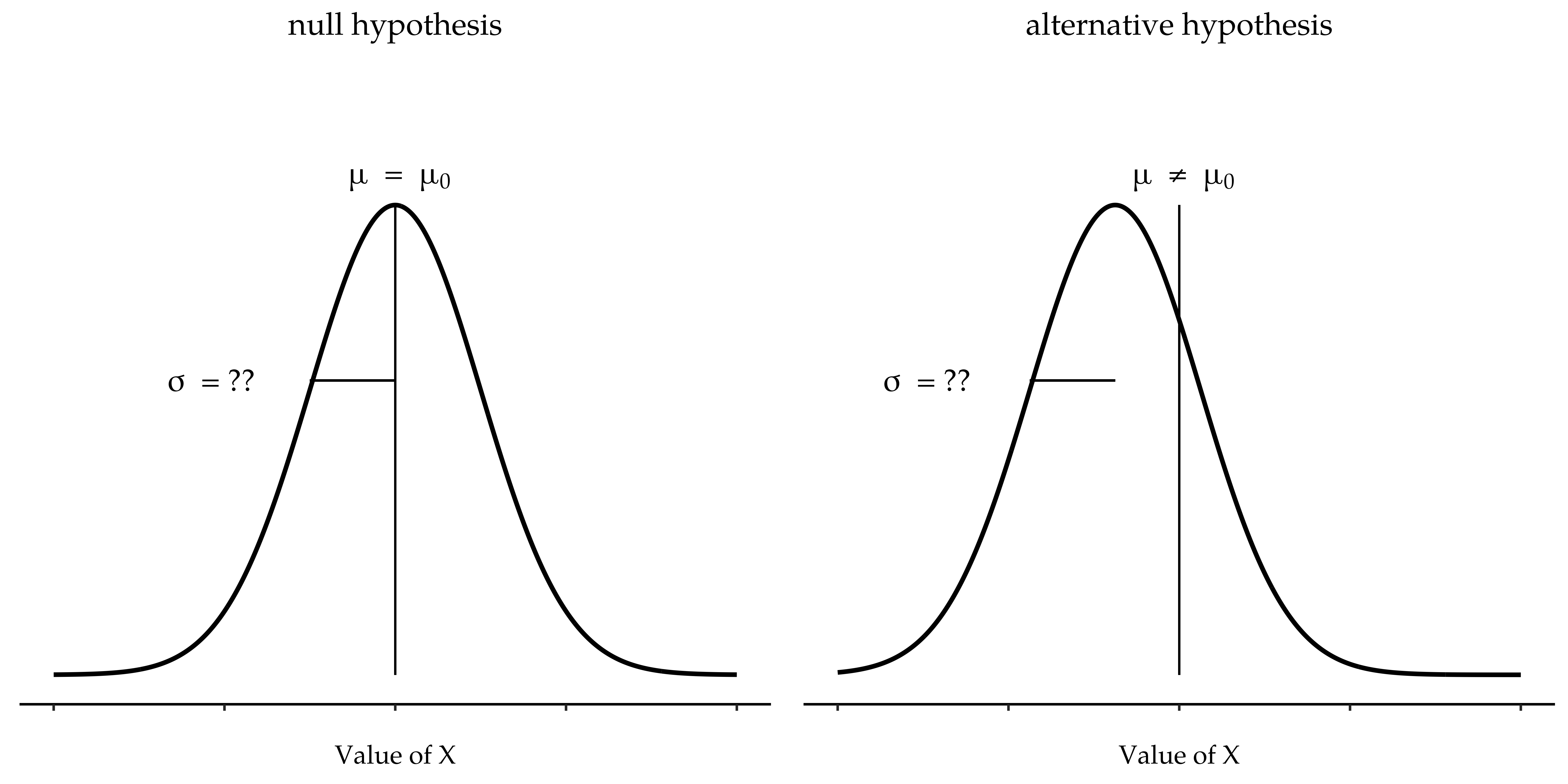
Fig. 100 Graphical illustration of the null and alternative hypotheses assumed by the (two-sided) one-sample t-test. Note the similarity to the z-test Fig. 98. The null hypothesis is that the population mean μ is equal to some specified value μ₀, and the alternative hypothesis is that it is not. Like the z-test, we assume that the data are normally distributed, but we do not assume that the population standard deviation σ is known in advance.

Vi introduserer t-testen

This ambiguity is annoying, and it was resolved in 1908 by a guy called William Sealy Gosset (Student, 1908), who was working as a chemist for the Guinness brewery at the time (Box, 1987). Because Guinness took a dim view of its employees publishing statistical analysis (apparently they felt it was a trade secret), he published the work under the pseudonym “A Student” and, to this day, the full name of the t-test is actually Student’s *t*-test. The key thing that Gosset figured out is how we should accommodate the fact that we are not completely sure what the true standard deviation is.[1] The answer is that it subtly changes the sampling distribution. In the t-test our test statistic, now called a t-statistic, is calculated in exactly the same way I mentioned above. If our null hypothesis is that the true mean is µ, but our sample has mean X̄ and our estimate of the population standard deviation is \(\hat{\sigma}\), then our t-statistic is:

\[t = \frac{\bar{X} - \mu}{\hat{\sigma}/\sqrt{N} }\]

The only thing that has changed in the equation is that instead of using the known true value σ, we use the estimate \(\hat{\sigma}\). And if this estimate has been constructed from N observations, then the sampling distribution turns into a t-distribution with N - 1 degrees of freedom (df). The t-distribution is very similar to the normal distribution, but has “heavier” tails, as discussed earlier in Andre nyttige distribusjoner and illustrated in Fig. 101. Notice, though, that as df gets larger, the t-distribution starts to look identical to the standard normal distribution. This is as it should be: if you have a sample size of N = 70 000 000 then your “estimate” of the standard deviation would be pretty much perfect, right? So, you should expect that for large N, the t-test would behave exactly the same way as a z-test. And that is exactly what happens!

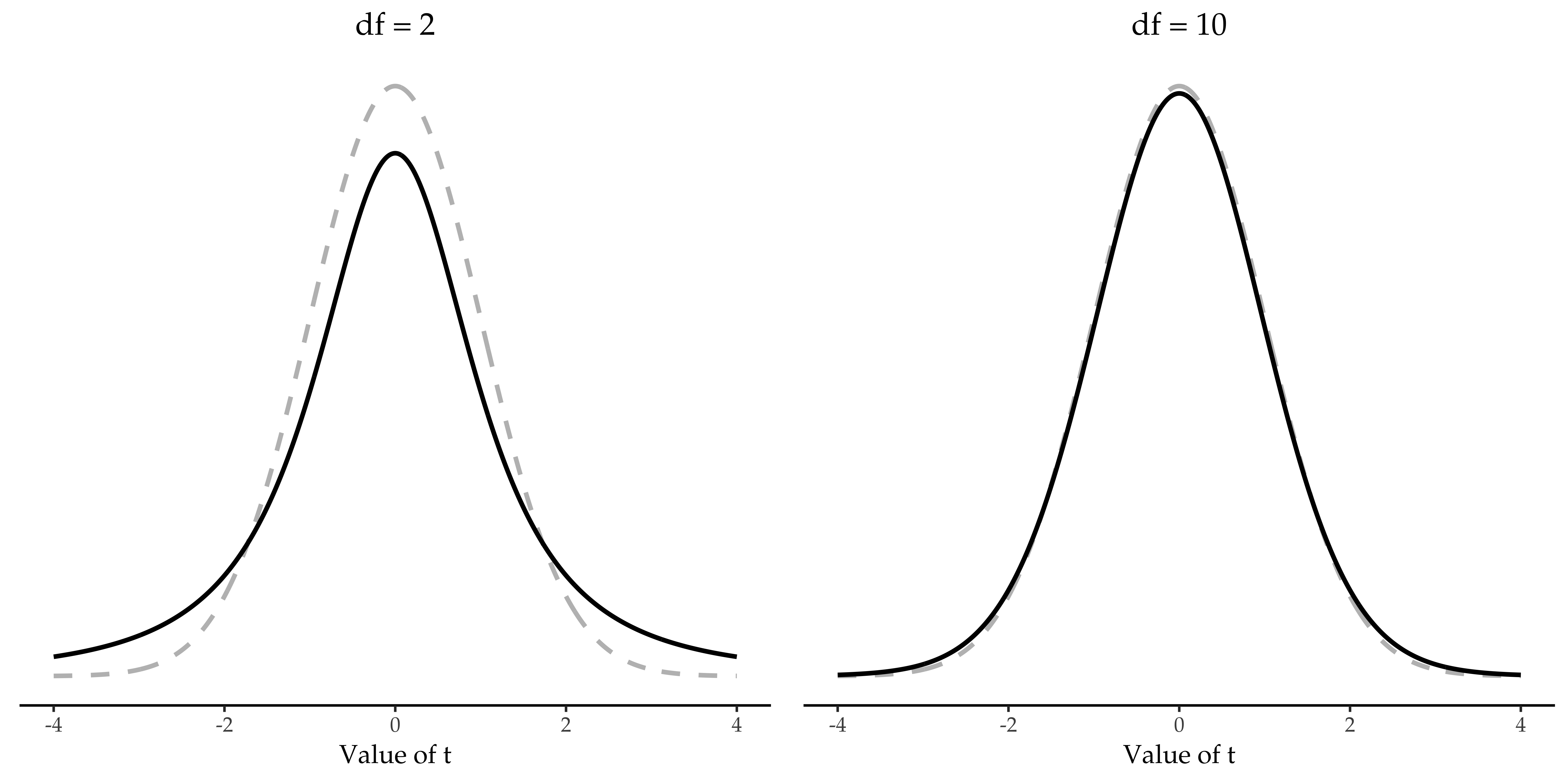
Fig. 101 t-fordelingen med 2 frihetsgrader (venstre panel) og 10 frihetsgrader (høyre panel), med en standard normalfordeling (dvs. gjennomsnitt = 0 og std. dev. = 1) plottet som stiplede linjer for sammenligningsformål. Legg merke til at t-fordelingen har tyngre haler (leptokurtisk: høyere kurtose) enn normalfordelingen; denne effekten er ganske overdrevet når frihetsgradene er svært små, men ubetydelig for større verdier. Med andre ord, for store df er t-fordelingen i hovedsak identisk med en normalfordeling.

Gjør testen i jamovi

As you might expect, the mechanics of the t-test are almost identical to the mechanics of the z-test. So there is not much point in going through the tedious exercise of showing you how to do the calculations using low level commands. It is pretty much identical to the calculations that we did earlier, except that we use the estimated standard deviation and then we test our hypothesis using the t-distribution rather than the normal distribution. And so instead of going through the calculations in tedious detail for a second time, I will jump straight to showing you how t-tests are actually done. jamovi comes with a dedicated analysis for t-tests that is very flexible (it can run lots of different kinds of t-tests). It is pretty straightforward to use; all you need to do is specify Analyses → T-Tests → One Sample T-Test, move the variable you are interested in (X) across into the Variables box, and type in the mean value for the null hypothesis (67.5) in the Hypothesis → Test value box. Easy enough (see Fig. 102, which, amongst other things that we will get to in a moment, gives you a t*statistic = 2.25, with 19 degrees of freedom and an associated *p-value of 0.036.

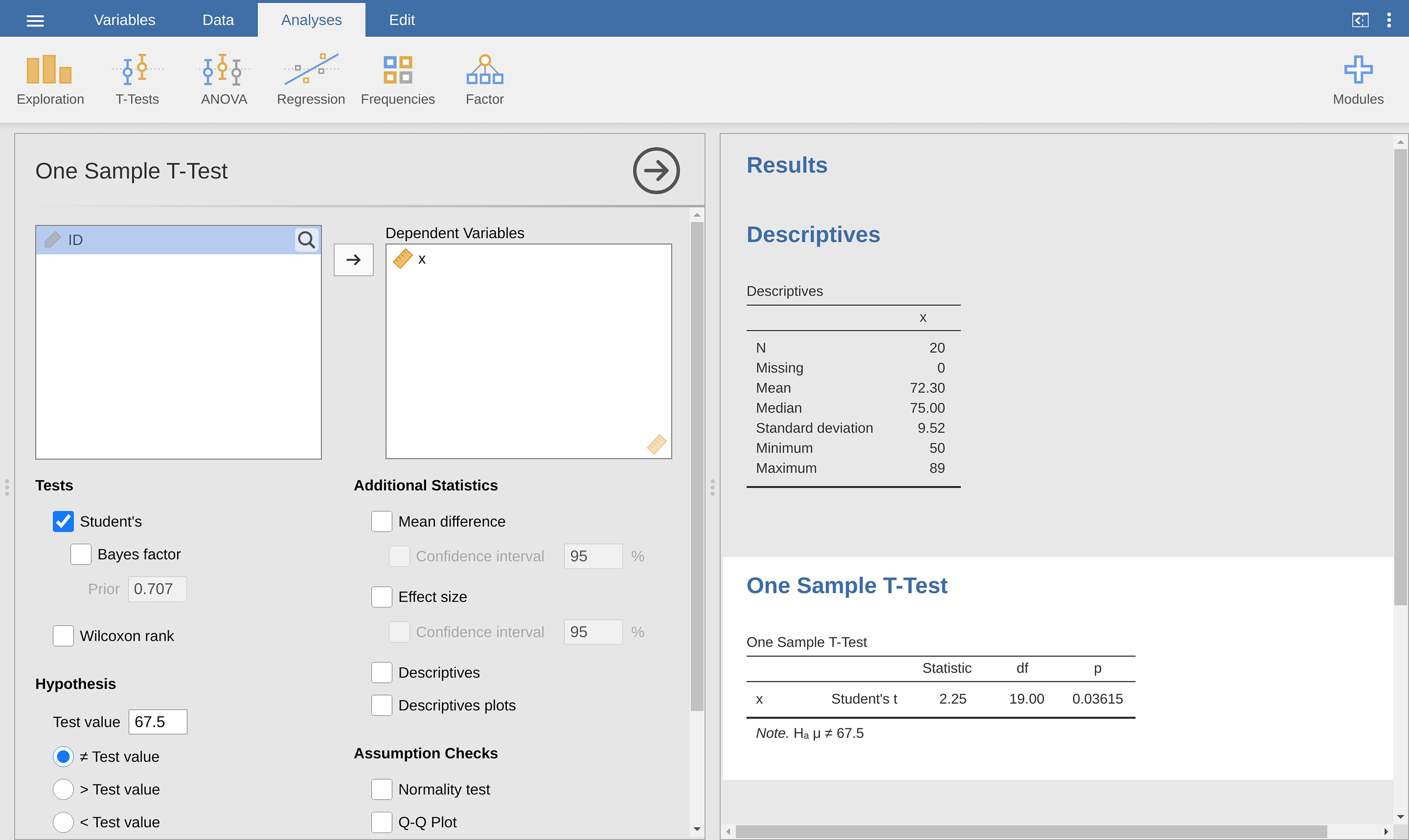
Fig. 102 Gjennomføring av en t-test med ett utvalg i jamovi

Also reported are two other things you might care about: the 95% confidence interval and a measure of effect size (we will talk more about effect sizes later). So that seems straightforward enough. Now what do we do with this output? Well, since we are pretending that we actually care about my toy example, we are overjoyed to discover that the result is statistically significant (i.e., a p-value below 0.05). We could report the result by saying something like this:

Med en gjennomsnittskarakter på 72,3 skåret psykologistudentene litt høyere enn gjennomsnittskarakteren på 67,5 (t(19) = 2,25, p < 0,05); gjennomsnittsforskjellen var 4,80 og konfidensintervallet på 95% var fra 0,34 til 9,26.

where t(19) is shorthand notation for a t-statistic that has 19 degrees of freedom. That said, it is often the case that people do not report the confidence interval, or do so using a much more compressed form than I have done here. For instance, it is not uncommon to see the confidence interval included as part of the stat block after reporting the mean difference, like this:

t(19) = 2.25, p = 0.036, CI₉₅ = [0.34, 9.26]

Med så mye sjargong stappet inn på en halv linje, vet du at det må være veldig smart.[2]

Forutsetninger for t-test med ett utvalg

Okay, so what assumptions does the one-sample t-test make? Well, since the t-test is basically a z-test with the assumption of known standard deviation removed, you should not be surprised to see that it makes the same assumptions as the z-test, minus the one about the known standard deviation. That is:

• Normality. We are still assuming that the population distribution is normal,[3] and as noted earlier, there are standard tools that you can use to check to see if this assumption is met (section Sjekk forutsetningen om normalfordeling for en stikkprøve), and other tests you can do in it is place if this assumption is violated (section Testing av ikke-normalfordelte data med Wilcoxon-tester).

• Uavhengighet. Igjen må vi anta at observasjonene i utvalget vårt er generert uavhengig av hverandre. Se den tidligere diskusjonen om z-testen for detaljer (avsnitt Forutsetninger for *z*-testen).

Overall, these two assumptions are not terribly unreasonable, and as a consequence the one-sample t-test is pretty widely used in practice as a way of comparing a sample mean against a hypothesised population mean.

---

[1]

Vel, på en måte. Slik jeg har forstått historien, leverte Gosset bare en delløsning; den generelle løsningen på problemet ble levert av Sir Ronald Fisher.

[2]

More seriously, I tend to think the reverse is true. I get very suspicious of technical reports that fill their results sections with nothing except the numbers. It might just be that I am an arrogant jerk, but I often feel like an author that makes no attempt to explain and interpret their analysis to the reader either does not understand it themselves, or is being a bit lazy. Your readers are smart, but not infinitely patient. Do not annoy them if you can help it.

[3]

A technical comment. In the same way that we can weaken the assumptions of the z-test so that we are only talking about the sampling distribution, we can weaken the t-test assumptions so that we do not have to assume normality of the population. However, for the t-test it is trickier to do this. As before, we can replace the assumption of population normality with an assumption that the sampling distribution of X̄ is normal. However, remember that we are also relying on a sample estimate of the standard deviation, and so we also require the sampling distribution of \(\hat{\sigma}\) to be χ². That makes things nastier, and this version is rarely used in practice. Fortunately, if the population distribution is normal, then both of these two assumptions are met.