Section author: Danielle J. Navarro and David R. Foxcroft

Repeated measures one-way ANOVA¶

The one-way repeated measures ANOVA test is a statistical method of testing for significant differences between three or more groups where the same participants are used in each group (or each participant is closely matched with participants in other experimental groups). For this reason, there should always be an equal number of scores (data points) in each experimental group. This type of design and analysis can also be called a “related ANOVA” or a “within-subjects ANOVA”.

The logic behind a repeated measures ANOVA is very similar to that of an independent ANOVA (sometimes called a “between-subjects” ANOVA). You’ll remember that earlier we showed that in a between-subjects ANOVA total variability is partitioned into between-groups variability (SS_b) and within-groups variability (SS_w), and after each is divided by the respective degrees of freedom to give MS_b and MS_w (see Table 16) the F-ratio is calculated as:

F = MS_b / MS_w

In a repeated measures ANOVA, the F-ratio is calculated in a similar way, but whereas in an independent ANOVA the within-group variability (SS_w) is used as the basis for the MS_w denominator, in a repeated measures ANOVA the SS_w is partioned into two parts. As we are using the same subjects in each group, we can remove the variability due to the individual differences between subjects (referred to as SS_subjects) from the within-groups variability. We won’t go into too much technical detail about how this is done, but essentially each subject becomes a level of a factor called subjects. The variability in this within-subjects factor is then calculated in the same way as any between-subjects factor. And then we can subtract SS_subjects from SS_w to provide a smaller SS_error term:

Independent ANOVA: SS_error = SS_w

Repeated Measures ANOVA: SS_error = SS_{w - SS:sub:`subjects}

This change in SS_error term often leads to a more powerful statistical test, but this does depend on whether the reduction in the SS_error more than compensates for the reduction in degrees of freedom for the error term: the degrees of freedom go from (n - k)[1] to (n - 1)(k - 1) remembering that there are more subjects in the independent ANOVA design.

Repeated measures ANOVA in jamovi¶

First, we need some data. Geschwind (1972) has suggested that the exact nature of a patient’s language deficit following a stroke can be used to diagnose the specific region of the brain that has been damaged. A researcher is concerned with identifying the specific communication difficulties experienced by six patients suffering from Broca’s Aphasia (a language deficit commonly experienced following a stroke).

Table 17 Number of attempts successfully completed on three experimental tasks.¶
Participant	Speech	Conceptual	Syntax
1	8	7	6
2	7	8	6
3	9	5	3
4	5	4	5
5	6	6	2
6	8	7	4

The patients were required to complete three word recognition tasks. On the first (speech production) task, patients were required to repeat single words read out aloud by the researcher. On the second (conceptual) task, designed to test word comprehension, patients were required to match a series of pictures with their correct name. On the third (syntax) task, designed to test knowledge of correct word order, patients were asked to reorder syntactically incorrect sentences. Each patient completed all three tasks. The order in which patients attempted the tasks was counterbalanced between participants. Each task consisted of a series of 10 attempts. The number of attempts successfully completed by each patient are shown in Table 17. Enter these data into jamovi ready for analysis (or take a short-cut and load the broca data set).

To perform a one-way related ANOVA in jamovi, open the one-way repeated measures ANOVA dialogue box, as in Fig. 138, via ANOVA - Repeated Measures ANOVA. Then:

Enter a name for the Repeated Measures Factors (orginally: RM Factor …). This should be a label that you choose to describe the conditions repeated by all participants. For example, to describe the speech, conceptual and syntax tasks completed by all participants a suitable label would be Task. Note that this new factor name represents the independent variable in the analysis.
Add a third level in the Repeated Measures Factors variable box, as there are three levels representing the three tasks: Speech, Conceptual and Syntax. Change the labels of the levels accordingly.
Then move each of the levels variables across to the Repeated Measures Cells text box.
Finally, under the Assumption Checks option, tick the Sphericity checks check box.

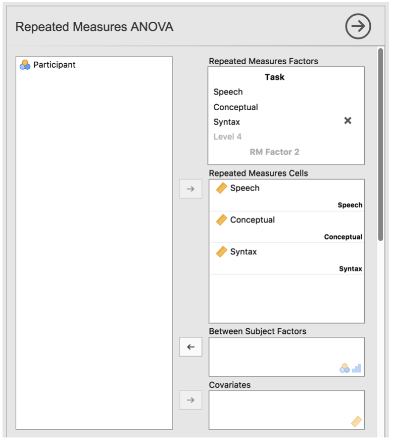
Fig. 138 Repeated measures ANOVA dialogue box in jamovi

jamovi output for a one-way Repeated Measures ANOVA is produced as shown in the Fig. 139 to Fig. 142. The first output we should look at is Mauchly’s Test of Sphericity, which tests the hypothesis that the variances of the differences between the conditions are equal (meaning that the spread of difference scores between the study conditions is approximately the same). In Fig. 139, Mauchly’s test significance level is p = 0.720. If Mauchly’s test is non-significant (i.e. p > 0.05, as is the case in this analysis) then it is reasonable to conclude that the variances of the differences are not significantly different (i.e. they are roughly equal and sphericity can be assumed.).

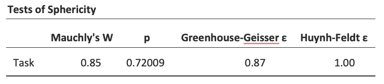
Fig. 139 One-way repeated measures ANOVA output: Mauchly’s Test of Sphericity

If, on the other hand, Mauchly’s test had been significant (p < 0.05) then we would conclude that there are significant differences between the variance of the differences, and the requirement of sphericity has not been met. In this case, we should apply a correction to the F-value obtained in the one-way related ANOVA analysis:

If the Greenhouse-Geisser value in the Tests of Sphericity table is > 0.75 then you should use the Huynh-Feldt correction.
But if the Greenhouse-Geisser value is < 0.75, then you should use the Greenhouse-Geisser correction.

Both these corrected F-values can be specified in the Sphericity Corrections check boxes under the Assumption Checks options, and the corrected F-values are then shown in the results table, as in Fig. 140.

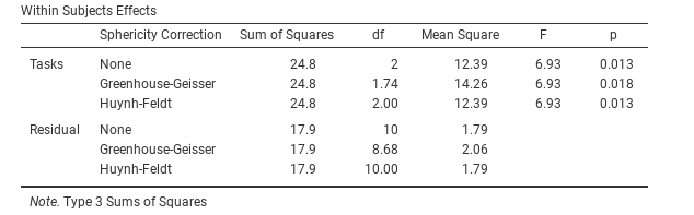
Fig. 140 One-way repeated measures ANOVA output: Tests of Within-Subjects Effects

In our analysis, we saw that the significance of Mauchly’s Test of Sphericity was p = 0.720 (i.e. p > 0.05). So, this means we can assume that the requirement of sphericity has been met so no correction to the F-value is needed. Therefore, we can use the None Sphericity Correction output values for the repeated measure Task: F = 6.93, df1 = 2, df2 = 10, p = 0.013, and we can conclude that the number of tests successfully completed on each language task did vary significantly depending on whether the task was speech, comprehension or syntax based (F(2,10) = 6.93, p = 0.013).

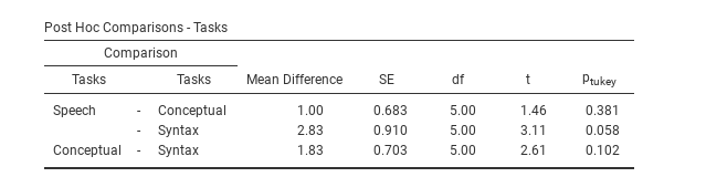
Fig. 141 Post-hoc tests in repeated measures ANOVA in jamovi

Post-hoc tests can also be specified in jamovi for repeated measures ANOVA in the same way as for independent ANOVA. The results are shown in Fig. 141. These indicate that there is a significant difference between Speech and Syntax, but not between other levels.

Descriptive statistics (marginal means) can be reviewed to help interpret the results, produced in the jamovi output as in Fig. 142. Comparison of the mean number of trials successfully completed by participants shows that Broca’s Aphasics perform reasonably well on speech production (mean = 7.17) and language comprehension (mean = 6.17) tasks. However, their performance was considerably worse on the syntax task (mean = 4.33), with a significant difference in post-hoc tests between Speech and Syntax task performance.

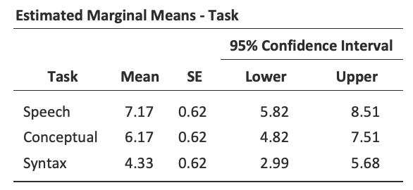
Fig. 142 One-way repeated measures ANOVA output: Descriptive Statistics

[1]	(n - k): (number of subjects - number of groups)