Section author: Danielle J. Navarro and David R. Foxcroft
Multiple comparisons and post-hoc tests
Any time you run an ANOVA with more than two groups and you end up with a significant effect, the first thing you’ll probably want to ask is which groups are actually different from one another. In our drugs example, our null hypothesis was that all three drugs (placebo, Anxifree and Joyzepam) have the exact same effect on mood. But if you think about it, the null hypothesis is actually claiming three different things all at once here. Specifically, it claims that:
- Your competitor’s drug (Anxifree) is no better than a placebo (i.e., µA = µP)
- Your drug (Joyzepam) is no better than a placebo (i.e., µJ = µP)
- Anxifree and Joyzepam are equally effective (i.e., µJ = µA)
If any one of those three claims is false, then the null hypothesis is also false. So, now that we’ve rejected our null hypothesis, we’re thinking that at least one of those things isn’t true. But which ones? All three of these propositions are of interest. Since you certainly want to know if your new drug Joyzepam is better than a placebo, it would be nice to know how well it stacks up against an existing commercial alternative (i.e., Anxifree). It would even be useful to check the performance of Anxifree against the placebo. Even if Anxifree has already been extensively tested against placebos by other researchers, it can still be very useful to check that your study is producing similar results to earlier work.
When we characterise the null hypothesis in terms of these three distinct propositions, it becomes clear that there are eight possible “states of the world” that we need to distinguish between:
| possibility: | is µP = µA | is µP = µJ | is µA = µJ | which hypothesis? |
|---|---|---|---|---|
| 1 | ✓ | ✓ | ✓ | null |
| 2 | ✓ | ✓ | alternative | |
| 3 | ✓ | ✓ | alternative | |
| 4 | ✓ | ✓ | alternative | |
| 5 | ✓ | alternative | ||
| 6 | ✓ | alternative | ||
| 7 | ✓ | alternative | ||
| 8 | alternative |
By rejecting the null hypothesis, we’ve decided that we don’t believe that #1 is the true state of the world. The next question to ask is, which of the other seven possibilities do we think is right? When faced with this situation, its usually helps to look at the data. For instance, if we look at the plots in Fig. 130, it’s tempting to conclude that Joyzepam is better than the placebo and better than Anxifree, but there’s no real difference between Anxifree and the placebo. However, if we want to get a clearer answer about this, it might help to run some tests.
Running “pairwise” t-tests
How might we go about solving our problem? Given that we’ve got three
separate pairs of means (placebo versus Anxifree, placebo versus
Joyzepam, and Anxifree versus Joyzepam) to compare, what we could do is
run three separate t-tests and see what happens. This is easy to do in
jamovi. Go to the ANOVA → Post Hoc Tests options, move the drug
variable across into the active box on the right, and then click on the
No correction checkbox. This will produce a neat table showing all the
pairwise t-test comparisons amongst the three levels of the
drug variable, as in Fig. 133.
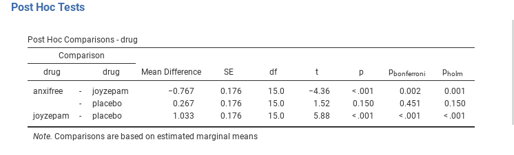
Fig. 133 Uncorrected pairwise t-tests as post-hoc comparisons in jamovi
Corrections for multiple testing
In the previous section I hinted that there’s a problem with just running lots and lots of t-tests. The concern is that, when running these analyses, what we’re doing is going on a “fishing expedition”. We’re running lots and lots of tests without much theoretical guidance in the hope that some of them come up significant. This kind of theory-free search for group differences is referred to as post-hoc analysis (“post-hoc” being Latin for “after this”).[1]
It’s okay to run post-hoc analyses, but a lot of care is required. For instance, the analysis that I ran in the previous section should be avoided, as each individual t-test is designed to have a 5% Type I error rate (i.e., α = 0.05) and I ran three of these tests. Imagine what would have happened if my ANOVA involved 10 different groups, and I had decided to run 45 “post-hoc” t-tests to try to find out which ones were significantly different from each other, you’d expect 2 or 3 of them to come up significant by chance alone. As we saw in chapter Hypothesis testing, the central organising principle behind null hypothesis testing is that we seek to control our Type I error rate, but now that I’m running lots of t-tests at once in order to determine the source of my ANOVA results, my actual Type I error rate across this whole family of tests has gotten completely out of control.
The usual solution to this problem is to introduce an adjustment to the p-value, which aims to control the total error rate across the family of tests (Shaffer, 1995). An adjustment of this form, which is usually (but not always) applied because one is doing post-hoc analysis, is often referred to as a correction for multiple comparisons, though it is sometimes referred to as “simultaneous inference”. In any case, there are quite a few different ways of doing this adjustment. I’ll discuss a few of them in this section and in section Post-hoc tests, but you should be aware that there are many other methods out there (Hsu, 1996).
Bonferroni corrections
The simplest of these adjustments is called the Bonferroni correction (Dunn, 1961), and it’s very very simple indeed. Suppose that my post-hoc analysis consists of m separate tests, and I want to ensure that the total probability of making any Type I errors at all is at most α.[2] If so, then the Bonferroni correction just says “multiply all your raw p-values by m”. If we let p denote the original p-value, and let p’j be the corrected value, then the Bonferroni correction tells that:
p’j = m × p
And therefore, if you’re using the Bonferroni correction, you would reject the null hypothesis if p’j < α. The logic behind this correction is very straightforward. We’re doing m different tests, so if we arrange it so that each test has a Type I error rate of at most α / m, then the total Type I error rate across these tests cannot be larger than α. That’s pretty simple, so much so that in the original paper, the author writes,
The method given here is so simple and so general that I am sure it must have been used before this. I do not find it, however, so can only conclude that perhaps its very simplicity has kept statisticians from realizing that it is a very good method in some situations (Dunn, 1961, pp. 52-53).
To use the Bonferroni correction in jamovi, just click on the
Bonferroni checkbox in the Correction options, and you will see
another column added to the ANOVA results table showing the adjusted
p-values for the Bonferroni correction (Fig. 133). If
we compare these three p-values to those for the uncorrected, pairwise
t-tests, it is clear that the only thing that jamovi has done is multiply
them by 3.
Holm corrections
Although the Bonferroni correction is the simplest adjustment out there, it’s not usually the best one to use. One method that is often used instead is the Holm correction (Holm, 1979). The idea behind the Holm correction is to pretend that you’re doing the tests sequentially, starting with the smallest (raw) p-value and moving onto the largest one. For the j-th largest of the p-values, the adjustment is either
p’j = j × pj
(i.e., the biggest p-value remains unchanged, the second biggest p-value is doubled, the third biggest p-value is tripled, and so on), or
p’j = p’j + 1
whichever one is larger. This might sound a little confusing, so let’s go through it a little more slowly. Here’s what the Holm correction does. First, you sort all of your p-values in order, from smallest to largest. For the smallest p-value all you do is multiply it by m, and you’re done. However, for all the other ones it’s a two-stage process. For instance, when you move to the second smallest p-value, you first multiply it by m - 1. If this produces a number that is bigger than the adjusted p-value that you got last time, then you keep it. But if it’s smaller than the last one, then you copy the last p-value. To illustrate how this works, consider the table below, which shows the calculations of a Holm correction for a collection of five p-values:
| raw p rank | j | p × j | Holm p |
|---|---|---|---|
| .001 | 5 | 0.005 | 0.005 |
| .005 | 4 | 0.020 | 0.020 |
| .019 | 3 | 0.057 | 0.057 |
| .022 | 2 | 0.044 | 0.057 |
| .103 | 1 | 0.103 | 0.103 |
Hopefully that makes things clear.
Although it’s a little harder to calculate, the Holm correction has some very nice properties. It’s more powerful than Bonferroni (i.e., it has a lower Type II error rate) but, counter-intuitive as it might seem, it has the same Type I error rate. As a consequence, in practice there’s never any reason to use the simpler Bonferroni correction since it is always outperformed by the slightly more elaborate Holm correction. Because of this, the Holm correction should be your go to multiple comparison correction. Fig. 133 also shows the Holm corrected p-values and, as you can see, the biggest p-value (corresponding to the comparison between Anxifree and the placebo) is unaltered. At a value of 0.15, it is exactly the same as the value we got originally when we applied no correction at all. In contrast, the smallest p-value (Joyzepam versus placebo) has been multiplied by three.
Writing up the post-hoc test
Finally, having run the post-hoc analysis to determine which groups are significantly different to one another, you might write up the result like this:
Post-hoc tests (using the Holm correction to adjust p) indicated that Joyzepam produced a significantly larger mood change than both Anxifree (p = 0.001) and the placebo (p = 9.0 · 10-5). We found no evidence that Anxifree performed better than the placebo (p = 0.15).
Or, if you don’t like the idea of reporting exact p-values, then you’d change those numbers to p < 0.001`, p < 0.01 and p > 0.05 respectively. Either way, the key thing is that you indicate that you used Holm’s correction to adjust the p-values. And of course, I’m assuming that elsewhere in the write up you’ve included the relevant descriptive statistics (i.e., the group means and standard deviations), since these p-values on their own aren’t terribly informative.
| [1] | If you do have some theoretical basis for wanting to investigate some comparisons but not others, it’s a different story. In those circumstances you’re not really running “post-hoc” analyses at all, you’re making “planned comparisons”. I do talk about this situation later in the book in section The method of planned comparisons), but for now I want to keep things simple. |
| [2] | It’s worth noting in passing that not all adjustment methods try to do this. What I’ve described here is an approach for controlling “family wise Type I error rate”. However, there are other post-hoc tests that seek to control the “false discovery rate”, which is a somewhat different thing. |