Auteur de la section : Danielle J. Navarro and David R. Foxcroft
Factorial ANOVA 2: balanced designs, interactions allowed
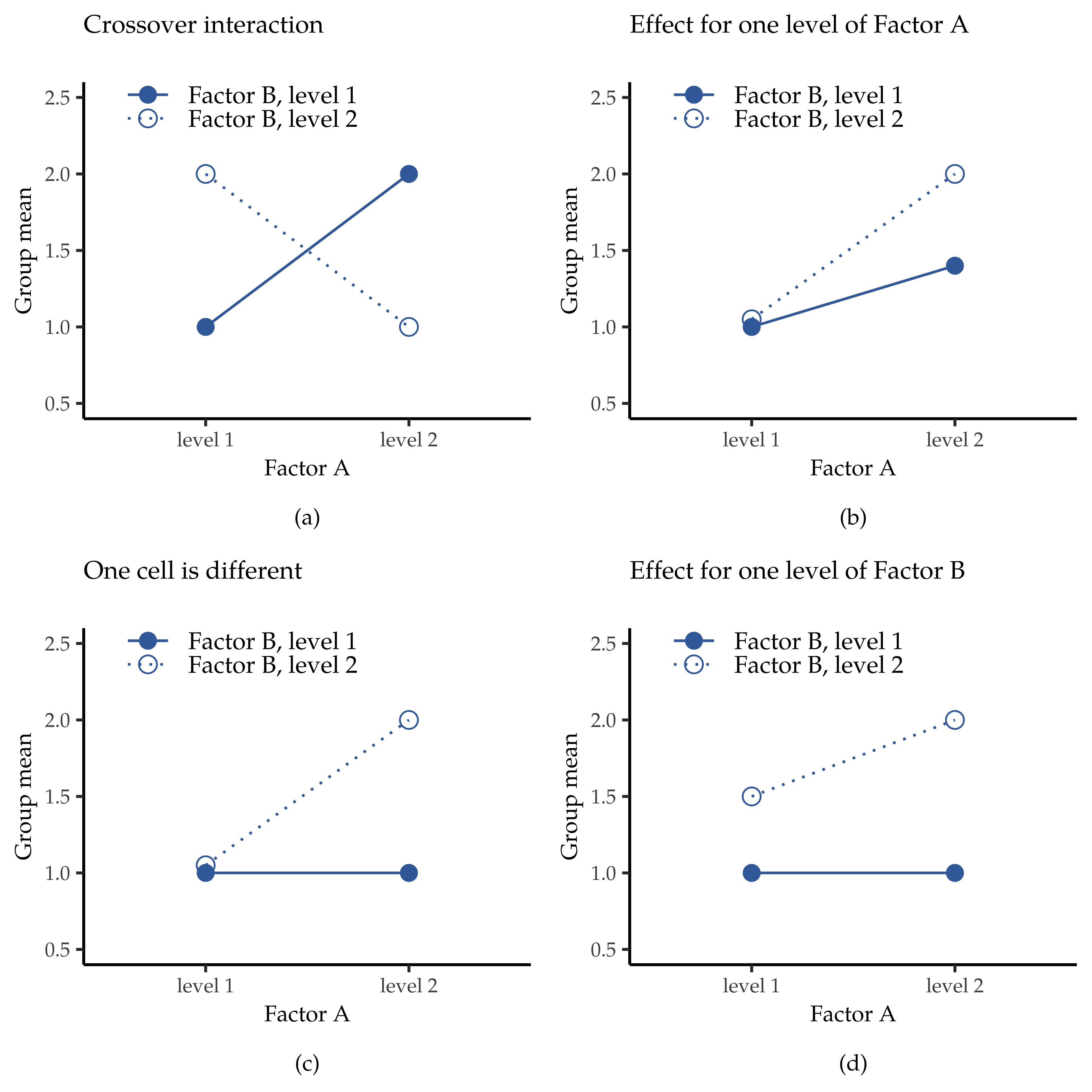
Fig. 170 Qualitatively different interactions for a 2 × 2 ANOVA
The four patterns of data shown in Fig. 169 are all quite realistic.
There are many data sets that produce exactly those patterns. However, they are
not the whole story and the ANOVA model that we have been talking about up to
this point is not sufficient to fully account for a table of group means. Why
not? Well, so far we have the ability to talk about the idea that drugs can
influence mood, and therapy can influence mood, but no way of talking about the
possibility of an interaction between the two. An interaction between A and
B is said to occur whenever the effect of factor A is different, depending on
which level of factor B we are talking about. Several examples of an interaction
effect with the context of a 2 × 2 ANOVA are shown in Fig. 170. To give
a more concrete example, suppose that the operation of Anxifree and Joyzepam is
governed by quite different physiological mechanisms. One consequence of this
is that while Joyzepam has more or less the same effect on mood regardless of
whether one is in therapy, Anxifree is actually much more effective when
administered in conjunction with CBT. The ANOVA that we developed in the
previous section does not capture this idea. To get some idea of whether there
actually is an interaction, it helps to plot the various group means. In jamovi
this is done via the ANOVA Estimated Marginal Means option – just move
drug and therapy across into the Marginal Means box under
Term 1. This should look something like Fig. 171.
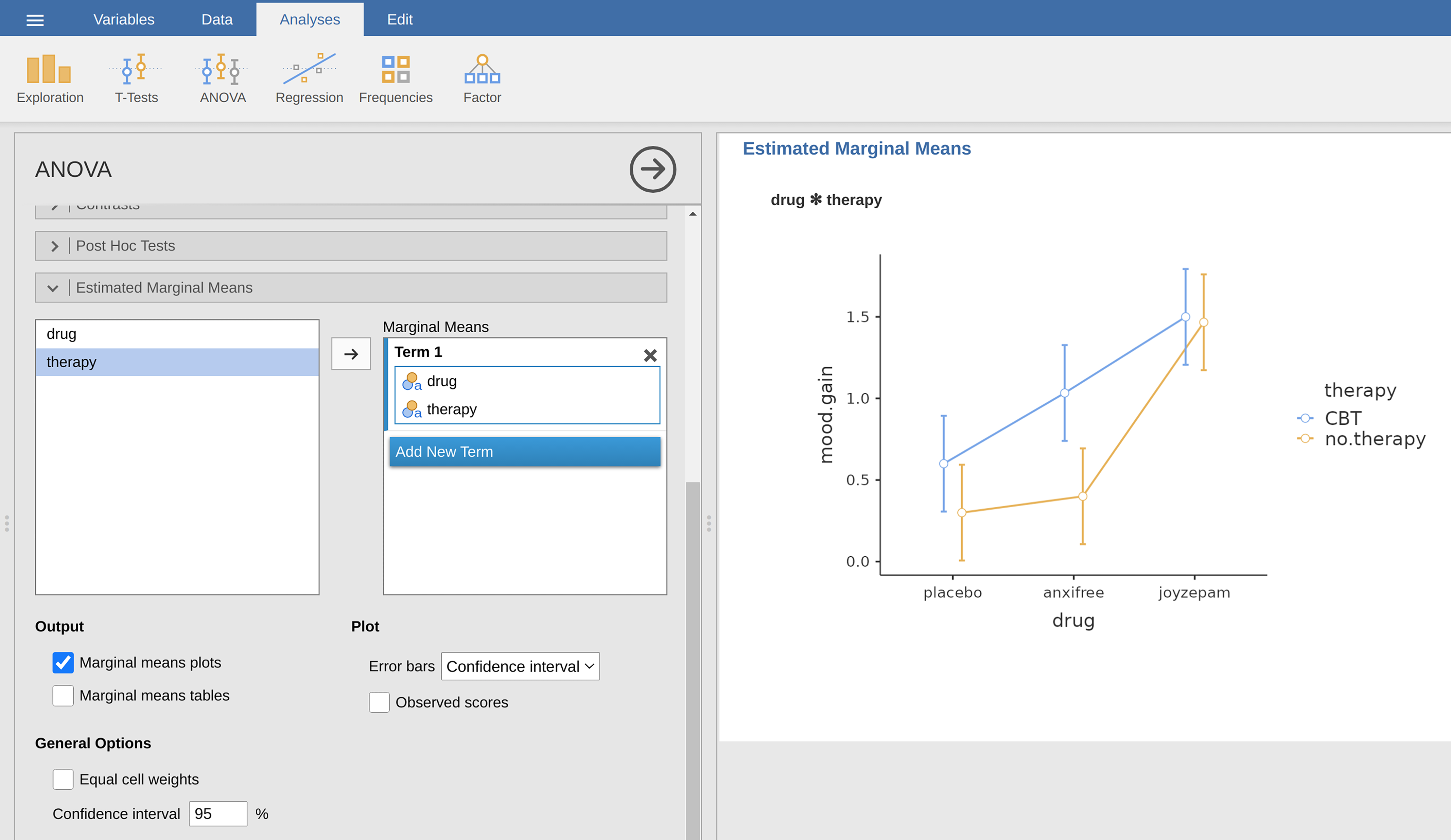
Fig. 171 jamovi screen shot showing how to generate a descriptive interaction plot
within the ANOVA (using Estimated Marginal Means) for the
clinicaltrial data set
Our main concern relates to the fact that the two lines are not parallel. The
effect of CBT (difference between solid line and dotted line) when the
drug is joyzepam (right side) appears to be near zero, even smaller
than the effect of CBT when a placebo is used (left side). However,
when anxifree is administered, the effect of CBT is larger than that of
no.therapy (middle). Is this effect real, or is this just random variation
due to chance? Our original ANOVA cannot answer this question, because we make
no allowances for the idea that interactions even exist! In this section, we
will fix this problem.
What exactly is an interaction effect?
The key idea that we are going to introduce in this section is that of an
interaction effect. In the ANOVA model we have looked at so far there are only
two factors involved in our model (i.e., drug and therapy). But when
we add an interaction we add a new component to the model: the combination of
drug and therapy. Intuitively, the idea behind an interaction effect is
fairly simple. It just means that the effect of factor A is different,
depending on which level of factor B we are talking about. But what does that
actually mean in terms of our data? The plot in Fig. 170 depicts
several different patterns that, although quite different to each other, would
all count as an interaction effect. So it is not entirely straightforward to
translate this qualitative idea into something mathematical that a statistician
can work with.
As a consequence, the way that the idea of an interaction effect is formalised in terms of null and alternative hypotheses is slightly difficult, and I am guessing that a lot of readers probably will not be that interested. Even so, I will try to give the basic idea here.
To start with, we need to be a little more explicit about our main effects.
Consider the main effect of factor A (drug in our running example). We
originally formulated this in terms of the null hypothesis that the two
marginal means µr. are all equal to each other. Obviously, if all of
these are equal to each other, then they must also be equal to the grand mean
µ.. as well, right? So what we can do is define the effect of factor
A at level r to be equal to the difference between the marginal mean
µr. and the grand mean µ... Let us denote this effect by
αr:
Now, by definition all of the αr values must sum to zero, for the same reason that the average of the marginal means µr. must be the grand mean µ... We can similarly define the effect of factor B at level i to be the difference between the column marginal mean µ.c and the grand mean µ..:
These βc values must sum to zero as well. The reason that statisticians sometimes like to talk about the main effects in terms of these αr and βc values is that it allows them to be precise about what it means to say that there is no interaction effect. If there is no interaction at all, then these αr and βc values will perfectly describe the group means µrc:
That is, there is nothing special about the group means that you could not predict perfectly by knowing all the marginal means. And that is our null hypothesis, right there. The alternative hypothesis is that for at least one group rc in our table:
However, statisticians often like to write this slightly differently. They will usually define the specific interaction associated with group rc to be some number, awkwardly referred to as αβrc, and then they will say that the alternative hypothesis is that αβrc is non-zero for at least one group:
This notation is kind of ugly to look at, but it is handy as we will see in the next section when discussing how to calculate the sum of squares.
Calculating sums of squares for the interaction
Calculating the sum of squares for an interaction term SSA:B is slightly trickier than the corresponding calculation for the main effects. The previous section defined the interaction effect in terms of the extent to which the actual group means differ from what you would expect by just looking at the marginal means. Of course, all of those formulas refer to population parameters rather than sample statistics, so we do not actually know what they are. However, we can estimate them by using sample means in place of population means. So for factor A, a good way to estimate the main effect at level r is as the difference between the sample marginal mean Ȳrc and the sample grand mean Ȳ... That is, we would use this as our estimate of the effect:
Similarly, our estimate of the main effect of factor B at level c can be defined as follows:
Now, if you go back to the formulas that I used to describe the SS values for the two main effects, you will notice that these effect terms are exactly the quantities that we were squaring and summing! The analogue for interaction terms can be found by first rearranging the formula for the group means µrc under the alternative hypothesis, so that we get this:
If we substitute our sample statistics in place of the population means, we get the following as our estimate of the interaction effect for group rc, which is:
Now all we have to do is sum all of these estimates across all r levels of factor A and all c levels of factor B, and we obtain the following formula for the sum of squares associated with the interaction as a whole:
We multiply by N because there are N observations in each of the groups, and we want our SS values to reflect the variation among observations accounted for by the interaction, not the variation among groups.
Now that we have a formula for calculating SSA:B, it is important to recognise that the interaction term is part of the model, so the total sum of squares associated with the model, SSM, is now equal to the sum of the three relevant SS values, SSA + SSB + SSA:B. The residual sum of squares SSR is still defined as the leftover variation, namely SST - SSM, but now that we have the interaction term this becomes:
As a consequence, the residual sum of squares SSR will be smaller than in our original ANOVA that did not include interactions.
Degrees of freedom for the interaction
Calculating the degrees of freedom for the interaction is slightly trickier than the corresponding calculation for the main effects. Let us start by thinking about the ANOVA model as a whole. Once we include interaction effects in the model we are allowing every single group to have a unique mean, µrc. For an r × c factorial ANOVA, this means that there are r × c quantities of interest in the model and only the one constraint: all of the group means need to average out to the grand mean. So the whole model needs to have (r × c) - 1 degrees of freedom. But the main effect of factor A has r - 1 degrees of freedom, and the main effect of factor B has c - 1 degrees of freedom. Therefore, the degrees of freedom for the interaction are the product of the degrees of freedom for the row factor and the column factor:
What about the residual degrees of freedom? Because we have added interaction terms which absorb some degrees of freedom, there are fewer residual degrees of freedom left over. Specifically, note that if the model with interaction has a total of (r × c) - 1, and there are N observations in your data set that are constrained to satisfy one grand mean, your residual degrees of freedom now become N -(r × c) - 1 + 1, or just N - (r × c).
Running the ANOVA in jamovi
Adding interaction terms to the ANOVA model in jamovi is straightforward. In
fact it is more than straightforward because it is the default option for
ANOVA. This means that when you specify an ANOVA with two factors, e.g.,
drug and therapy then the interaction component – drug ×
therapy (shown as drug * therapy) – is added automatically to the
model.[1] When we run the ANOVA with the interaction term included, then we
get the results shown in Fig. 172.
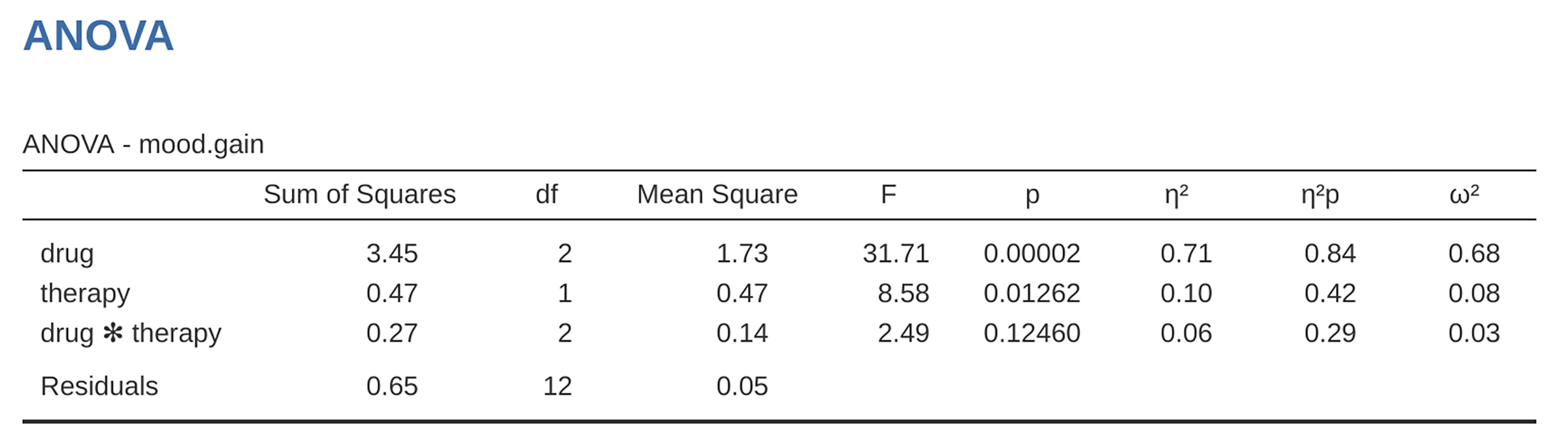
Fig. 172 Results for the full factorial model, including the interaction component
drug × therapy
As it turns out, while we do have a significant main effect of drug:
F(2,12) = 31.7, p < 0.001, and therapy: F(1,12) = 8.6, p =
0.013), there is no significant interaction between the two: F(2,12) = 2.5,
p = 0.125).
Interpreting the results
There is a couple of very important things to consider when interpreting the
results of factorial ANOVA. First, there is the same issue that we had with
one-way ANOVA, which is that if you obtain a significant main effect of (say)
drug, it does not tell you anything about how the levels of drug are
different to one another. To find that out, you need to run additional
analyses. We will talk about some analyses that you can run in sections
Different ways to specify contrasts and Post-hoc tests. The same is true for
interaction effects. Knowing that there is a significant interaction does not
tell you anything about what kind of interaction exists. Again, you will need
to run additional analyses.
Secondly, there is a very peculiar interpretation issue that arises when you obtain a significant interaction effect but no corresponding main effect. This happens sometimes. For instance, in the crossover interaction shown in Fig. 170 (a), this is exactly what you would find. In this case, neither of the main effects would be significant, but the interaction effect would be. This is a difficult situation to interpret, and people often get a bit confused about it. The general advice that statisticians like to give in this situation is that you should not pay much attention to the main effects when an interaction is present. The reason they say this is that, although the tests of the main effects are perfectly valid from a mathematical point of view, when there is a significant interaction effect the main effects rarely test interesting hypotheses. Recall from section What hypotheses are we testing? that the null hypothesis for a main effect is that the marginal means are equal to each other, and that a marginal mean is formed by averaging across several different groups. But if you have a significant interaction effect then you know that the groups that comprise the marginal mean are not homogeneous, so it is not really obvious why you would even care about those marginal means.
Here is what I mean. Again, let us stick with a clinical example. Suppose that
we had a 2 × 2 design comparing two different treatments for phobias (e.g.,
systematic desensitisation vs. flooding), and two different anxiety reducing
drugs (e.g., Anxifree vs Joyzepam). Now, suppose what we found was that
Anxifree had no effect when desensitisation was the treatment, and Joyzepam had
no effect when flooding was the treatment. But both were pretty effective for
the other treatment. This is a classic crossover interaction, and what we would
find when running the ANOVA is that there is no main effect of drug, but
a significant interaction. Now, what does it actually mean to say that
there is no main effect? Well, it means that if we average over the two
different psychological treatments, then the average effect of Anxifree and
Joyzepam is the same. But why would anyone care about that? When treating
someone for phobias it is never the case that a person can be treated using an
“average” of flooding and desensitisation. That does not make a lot of sense.
You either get one or the other. For one treatment one drug is effective, and
for the other treatment the other drug is effective. The interaction is the
important thing and the main effect is kind of irrelevant.
This sort of thing happens a lot. The main effect are tests of marginal means, and when an interaction is present we often find ourselves not being terribly interested in marginal means because they imply averaging over things that the interaction tells us should not be averaged! Of course, it is not always the case that a main effect is meaningless when an interaction is present. Often you can get a big main effect and a very small interaction, in which case you can still say things like “drug A is generally more effective than drug B” (because there was a big effect of drug), but you would need to modify it a bit by adding that “the difference in effectiveness was different for different psychological treatments”. In any case, the main point here is that whenever you get a significant interaction you should stop and think about what the main effect actually means in this context. Do not automatically assume that the main effect is interesting.