Auteur de la section : Danielle J. Navarro and David R. Foxcroft

Assumptions of the one-way ANOVA

Like any statistical test, analysis of variance relies on some assumptions about the data, specifically the residuals. There are three key assumptions that you need to be aware of: normality, homogeneity of variance and independence.

If you remember back to subsection The model for the data and the meaning of *F* which I hope you at least skimmed even if you did not read the whole thing, I described the statistical models underpinning ANOVA in this way:

H₀: Y_ik = µ + ϵ_ik

H₁: Y_ik = µ_k + ϵ_ik

In these equations µ refers to a single grand population mean which is the same for all groups, and µ_k is the population mean for the k-th group. Up to this point we have been mostly interested in whether our data are best described in terms of a single grand mean (the null hypothesis) or in terms of different group-specific means (the alternative hypothesis). This makes sense, of course, as that is actually the important research question! However, all of our testing procedures have, implicitly, relied on a specific assumption about the residuals, ϵ_ik, namely that

ϵ_ik ~ Normal(0, σ²)

None of the maths works properly without this bit. Or, to be precise, you can still do all the calculations and you will end up with an F-statistic, but you have no guarantee that this F-statistic actually measures what you think it is measuring, and so any conclusions that you might draw on the basis of the F test might be wrong.

So, how do we check whether the assumption about the residuals is accurate? Well, as I indicated above, there are three distinct claims buried in this one statement, and we will consider them separately.

• Homogeneity of variance. Notice that we have only got the one value for the population standard deviation (i.e., σ), rather than allowing each group to have it is own value (i.e., σ_k). This is referred to as the homogeneity of variance (sometimes called homoscedasticity) assumption. ANOVA assumes that the population standard deviation is the same for all groups. We will talk about this extensively in subsection Checking the homogeneity of variance assumption.

• Normality. The residuals are assumed to be normally distributed. As we saw in subsection Checking the normality of a sample, we can assess this by looking at QQ-plots (or running a Shapiro-Wilk test). I will talk about this more in an ANOVA context in subsection Checking the normality assumption.

• Independence. The independence assumption is a little trickier. What it basically means is that, knowing one residual tells you nothing about any other residual. All of the ϵ_ik values are assumed to have been generated without any “regard for” or “relationship to” any of the other ones. There is not an obvious or simple way to test for this, but there are some situations that are clear violations of this. For instance, if you have a repeated-measures design, where each participant in your study appears in more than one condition, then independence does not hold. There is a special relationship between some observations, namely those that correspond to the same person! When that happens, you need to use something like repeated measures ANOVA (see section Repeated measures one-way ANOVA).

Checking the homogeneity of variance assumption

There is more than one way to test the homogeneity of variance assumption, too (though for some reason no-one made a saying out of that). The most commonly used test for this that I have seen in the literature is the Levene test (Levene, 1960), and the closely related Brown-Forsythe test (Brown & Forsythe, 1974).

Regardless of whether you are doing the standard Levene test or the Brown-Forsythe test, the test statistic, which is sometimes denoted F but also sometimes written as W, is calculated in exactly the same way that the F-statistic for the regular ANOVA is calculated, just using a Z_ik rather than Y_ik. With that in mind, we can go on to look at how to run the test in jamovi.

The Levene test is shockingly simple. Suppose we have our outcome variable Y_ik. All we do is define a new variable, which I will call Z_ik, corresponding to the absolute deviation from the group mean:

Z_ik = Y_ik - Ȳ_k

Okay, what good does this do us? Well, let us take a moment to think about what Z_ik actually is and what we are trying to test. The value of Z_ik is a measure of how the i-th observation in the k-th group deviates from its group mean. And our null hypothesis is that all groups have the same variance, i.e., the same overall deviations from the group means! So the null hypothesis in a Levene test is that the population means of Z are identical for all groups. Hmm. So what we need now is a statistical test of the null hypothesis that all group means are identical. Where have we seen that before? Oh right, that is what ANOVA is, and so all that the Levene test does is run an ANOVA on the new variable Z_ik.

What about the Brown-Forsythe test? Does that do anything particularly different? Nope. The only change from the Levene test is that it constructs the transformed variable Z in a slightly different way, using deviations from the group medians (Md) rather than deviations from the group means. That is, for the Brown-Forsythe test (where Md_k(Y) is the median for group k):

Z_ik = Y_ik - Md_k(Y)

Running the Levene-test in jamovi

Okay, so how do we run the Levene test? Under the ANOVA → Assumption Checks option, just click on the Homogeneity tests checkbox. If we look at the output, shown in Fig. 156, we see that the test is non-significant: F(2,15) = 1.45, p = 0.266. So it looks like the homogeneity of variance assumption is fine. However, looks can be deceptive! If your sample size is pretty big, then the Levene test could show up a significant effect (i.e., p < 0.05) even when the homogeneity of variance assumption is not violated to an extent which troubles the robustness of ANOVA. This was the point George Box was making in the quote above. Similarly, if your sample size is quite small, then the homogeneity of variance assumption might not be satisfied and yet a Levene test could be non-significant (i.e., p > 0.05). What this means is that, alongside any statistical test of the assumption being met, you should always plot the standard deviation around the means for each group / category in the analysis… just to see if they look fairly similar (i.e., homogeneity of variance) or not.

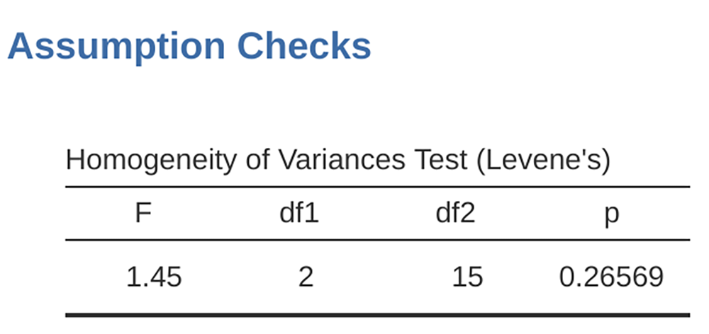
Fig. 156 Levene test output for One-Way ANOVA in jamovi

Removing the homogeneity of variance assumption

In our example, the homogeneity of variance assumption turned out to be a pretty safe one: the Levene test came back non-significant (notwithstanding that we should also look at the plot of standard deviations), so we probably do not need to worry. However, in real life we are not always that lucky. How do we save our ANOVA when the homogeneity of variance assumption is violated? If you recall from our discussion of t-tests, we have seen this problem before. The Student t-test assumes equal variances, so the solution was to use the Welch t-test, which does not. In fact, Welch (1951) also showed how we can solve this problem for ANOVA too (the Welch One-way test). It is implemented in jamovi using the One-Way ANOVA analysis. This is a specific analysis approach just for one-way ANOVA, and to run the Welch one-way ANOVA for our example, we would re-run the analysis as previously, but this time use the jamovi ANOVA → One Way ANOVA analysis command, and check the option Don't assume equal (Welch’s) (see Fig. 157).

Fig. 157 Welch’s test as part of the One-Way ANOVA analysis in jamovi

To understand what is happening here, let us compare these numbers with those obtained earlier in section Running an ANOVA in jamovi, namely: F(2,15) = 18.611, p = 0.00009. As shown in Fig. 157, these values are also displayed in the One-Way ANOVA table (in the row starting with Fisher's) if the option Assume equal (Fisher's) was chosen.

Okay, so originally our ANOVA gave us the result F(2,15) = 18.6, whereas the Welch one-way test gave us F(2,9.49) = 26.32. In other words, the Welch test has reduced the within-groups degrees of freedom from 15 to 9.49, and the F-value has increased from 18.6 to 26.32.

Checking the normality assumption

Testing the normality assumption is relatively straightforward. We covered most of what you need to know in section Checking the normality of a sample. The only thing we really need to do is draw a QQ plot and, in addition if it is available, run the Shapiro-Wilk test. The QQ plot is shown in Fig. 158 and it looks pretty normal to me. If the Shapiro-Wilk test is not significant (i.e., p > 0.05) then this indicates that the assumption of normality is not violated. However, as with Levene’s test, if the sample size is large then a significant Shapiro-Wilk test may in fact be a false positive, where the assumption of normality is not violated in any substantive problematic sense for the analysis. And, similarly, a very small sample can produce false negatives. That is why a visual inspection of the QQ plot is important.

Alongside inspecting the QQ plot for any deviations from normality, the Shapiro-Wilk test for our data does show a non-significant effect, with p = 0.6053 (see Fig. 157). This therefore supports the QQ plot assessment; both checks find no indication that normality is violated.

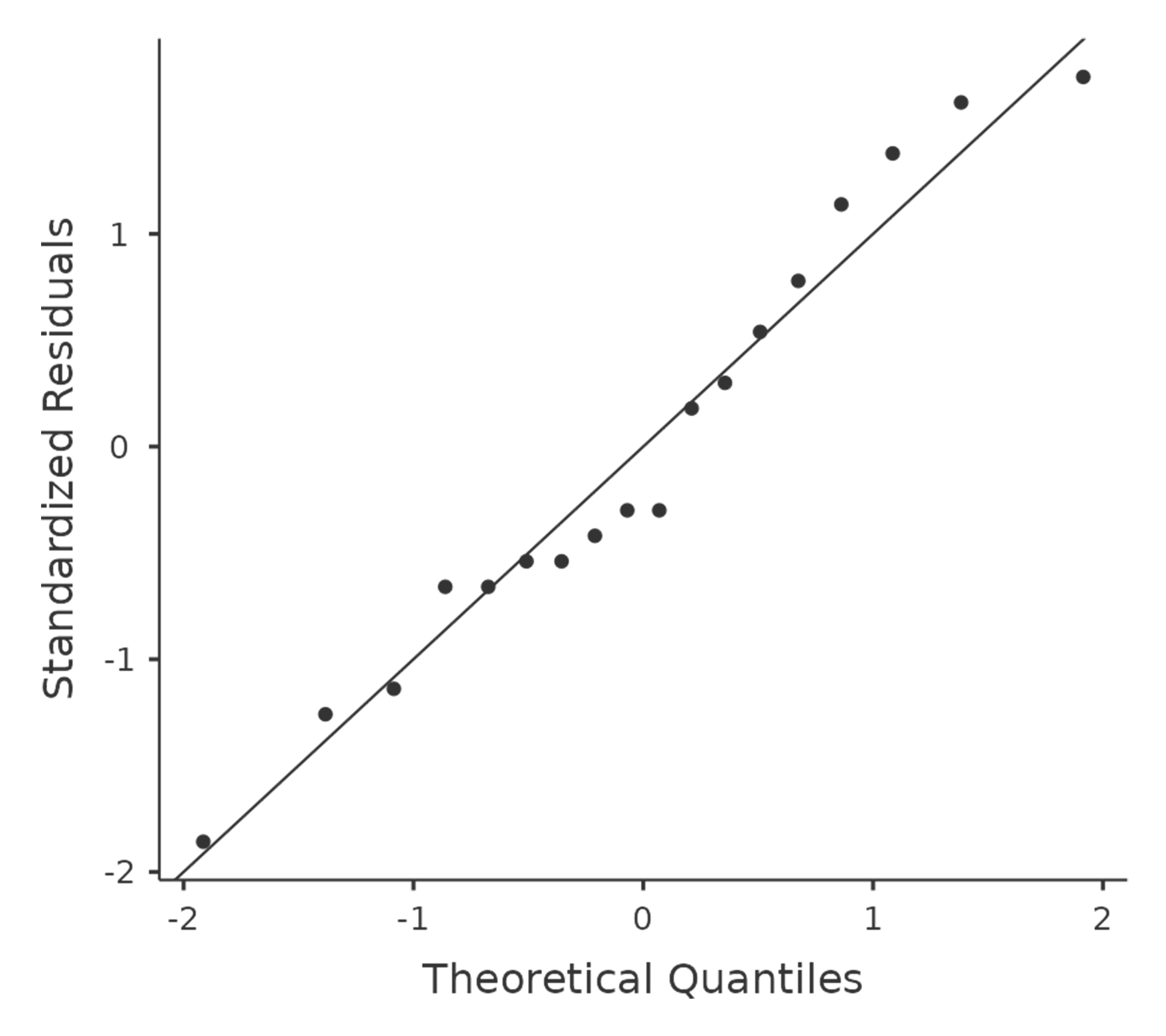
Fig. 158 QQ-plot produced from jamovi One-Way ANOVA options

Removing the normality assumption

Now that we have seen how to check for normality, we are led naturally to ask what we can do to address violations of normality. In the context of a One-way ANOVA, the easiest solution is probably to switch to a non-parametric test (i.e., one that does not rely on any particular assumption about the kind of distribution involved). We have seen non-parametric tests before, in section Testing non-normal data with Wilcoxon tests. When you only have two groups, the Mann-Whitney or the Wilcoxon test provides the non-parametric alternative that you need. When you have got three or more groups, you can use the Kruskal-Wallis rank sum test (Kruskal & Wallis, 1952). So that is the test we will talk about next.

The Kruskal-Wallis test is surprisingly similar to ANOVA, in some ways. In ANOVA we started with Y_ik, the value of the outcome variable for the i-th person in the k-th group. For the Kruskal-Wallis test what we will do is rank order all of these Y_ik values and conduct our analysis on the ranked data.

So let us let R_ik refer to the ranking given to the i-th member of the k-th group. Now, let us calculate R̄_k, the average rank given to observations in the k-th group:

\[\bar{R}_k = \frac{1}{N_K} \sum_{i} R_{ik}\]

and let us also calculate R̄, the grand mean rank

\[\bar{R} = \frac{1}{N} \sum_{i} \sum_{k} R_{ik}\]

Now that we have done this, we can calculate the squared deviations from the grand mean rank R̄. When we do this for the individual scores, i.e., if we calculate (R_ik – R̄)², what we have is a “non-parametric” measure of how far the ik-th observation deviates from the grand mean rank. When we calculate the squared deviation of the group means from the grand means, i.e., if we calculate (R̄_k – R̄)², then what we have is a non-parametric measure of how much the group deviates from the grand mean rank. With this in mind, we will follow the same logic that we did with ANOVA and define our ranked sums of squares measures, much like we did earlier. First, we have our “total ranked sums of squares”

\[\mbox{RSS}_{tot} = \sum_k \sum_i ( R_{ik} - \bar{R} ) ^ 2\]

and we can define the “between groups ranked sums of squares” like this:

\[\begin{split}\begin{array}{rcl} \mbox{RSS}_{b} &=& \sum_k \sum_i (\bar{R}_k - \bar{R}) ^ 2 \\ &=& \sum_k N_k (\bar{R}_k - \bar{R}) ^ 2 \end{array}\end{split}\]

So, if the null hypothesis is true and there are no true group differences at all, you would expect the between group rank sums RSS_b to be very small, much smaller than the total rank sums RSS_tot. Qualitatively this is very much the same as what we found when we went about constructing the ANOVA F-statistic, but for technical reasons the Kruskal-Wallis test statistic, usually denoted K, is constructed in a slightly different way,

\[K = (N - 1) \times \frac{\mbox{RSS}_b}{\mbox{RSS}_{tot}}\]

and if the null hypothesis is true, then the sampling distribution of K is approximately χ² with G - 1 degrees of freedom (where G is the number of groups). The larger the value of K, the less consistent the data are with the null hypothesis, so this is a one-sided test. We reject H₀ when K is sufficiently large.

The description in the previous section illustrates the logic behind the Kruskal-Wallis test. At a conceptual level, this is the right way to think about how the test works. However, from a purely mathematical perspective it is needlessly complicated. I will not show you the derivation, but you can use a bit of algebraic jiggery-pokery [1] to show that the equation for K can be rewritten as

\[K = \frac{12}{N(N - 1)} \sum_k N_k {\bar{R}_k} ^ 2 - 3(N + 1)\]

It is this last equation that you sometimes see given for K. This is way easier to calculate than the version I described in the previous section, but it is just that it is totally meaningless to actual humans. It is probably best to think of K the way I described it earlier, as an analogue of ANOVA based on ranks. But keep in mind that the test statistic that gets calculated ends up with a rather different look to it than the one we used for our original ANOVA.

But wait, there is more! Dear lord, why is there always more? The story I have told so far is only actually true when there are no ties in the raw data. That is, if there are no two observations that have exactly the same value. If there are ties, then we have to introduce a correction factor to these calculations. At this point I am assuming that even the most diligent reader has stopped caring (or at least formed the opinion that the tie-correction factor is something that does not require their immediate attention). So I will very quickly tell you how it is calculated, and omit the tedious details about why it is done this way. Suppose we construct a frequency table for the raw data, and let f_j be the number of observations that have the j-th unique value. This might sound a bit abstract, so here is a concrete example from the frequency table of mood.gain from the clinicaltrial data set:

0.1	0.2	0.3	0.4	0.5	0.6	0.8	0.9	1.1	1.2	1.3	1.4	1.7	1.8
1	1	2	1	1	2	1	1	1	1	2	2	1	1

Looking at this table, notice that the third entry in the frequency table has a value of 2. Since this corresponds to a mood.gain of 0.3, this table is telling us that two people’s mood increased by 0.3. More to the point, in the mathematical notation I introduced above, this is telling us that f₃ = 2. So, now that we know this, the tie correction factor (TCF) is:

\[\mbox{TCF} = 1 - \frac{\sum_j {f_j} ^ 3 - f_j}{N ^ 3 - N}\]

The tie-corrected value of the Kruskal-Wallis statistic is obtained by dividing the value of K by this quantity. It is this tie-corrected version that jamovi calculates. And at long last, we are actually finished with the theory of the Kruskal-Wallis test. I am sure you are all terribly relieved that I have cured you of the existential anxiety that naturally arises when you realise that you do not know how to calculate the tie-correction factor for the Kruskal-Wallis test.

How to run the Kruskal-Wallis test in jamovi

Despite the horror that we have gone through in trying to understand what the Kruskal-Wallis test actually does, it turns out that running the test is pretty painless, since jamovi has an analysis as part of the ANOVA analysis set called Non-Parametric → One-Way ANOVA (Kruskall-Wallis). Most of the time, you will have data like the clinicaltrial data set, in which you have your outcome variable mood.gain and a grouping variable drug. If so, you can just go ahead and run the analysis in jamovi. What this gives us is a Kruskal-Wallis χ² = 12.076, df = 2, p-value = 0.00239, as in Fig. 159.

Fig. 159 Non-parametric One-Way ANOVA (Kruskal-Wallis) in jamovi

---

[1]

A technical term.