Auteur de la section : Danielle J. Navarro and David R. Foxcroft

Estimating a linear regression model

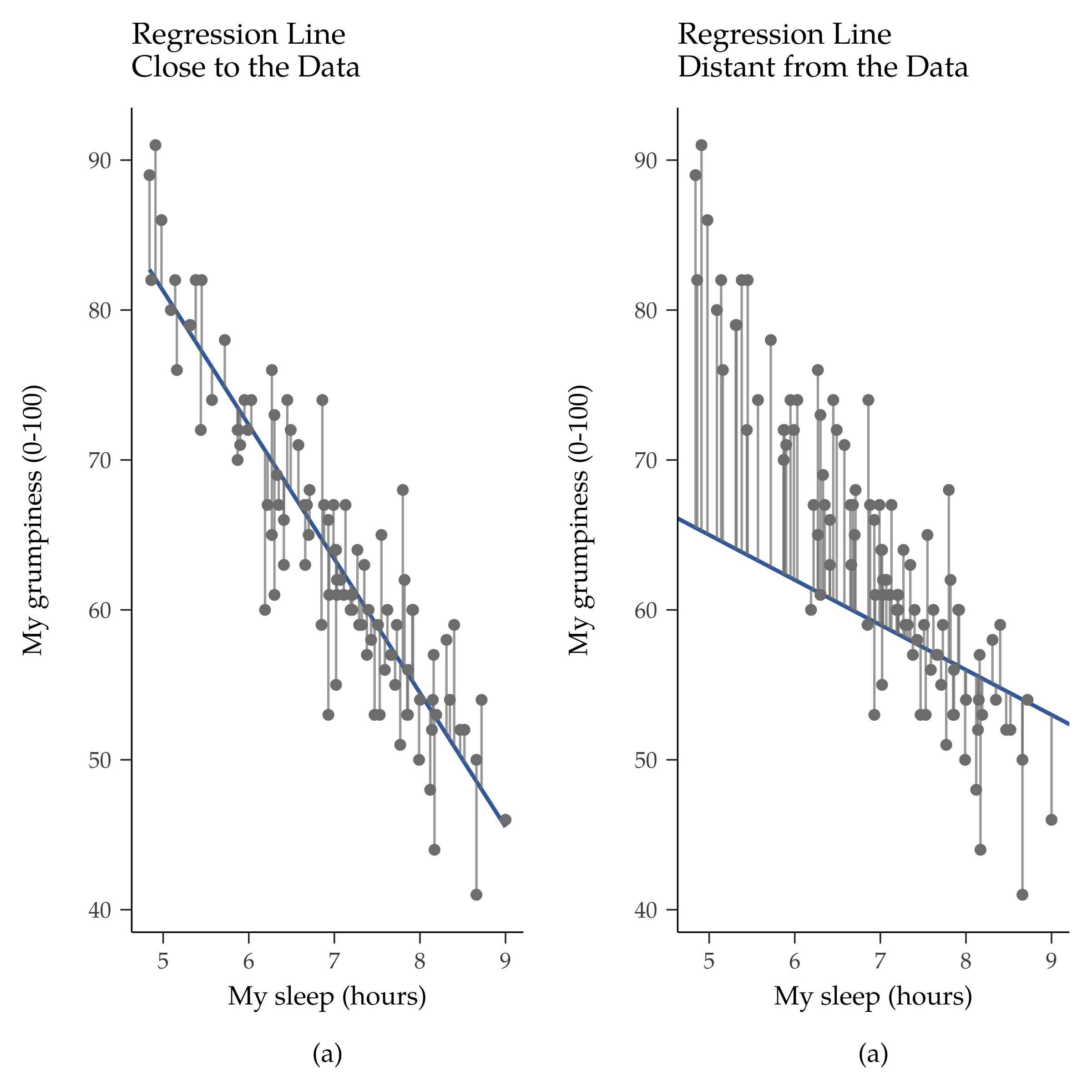
Fig. 135 Depiction of the residuals associated with the best fitting regression line (panel a), and the residuals associated with a poor regression line (panel b). The residuals are much smaller for the good regression line. Again, this is no surprise given that the good line is the one that goes right through the middle of the data.

Let us redraw our pictures but this time I will add some lines to show the size of the residual for all observations. When the regression line is good, our residuals (the lengths of the solid black lines) all look pretty small, as shown in Fig. 135 (a), but when the regression line is a bad one the residuals are a lot larger, as you can see from looking at Fig. 135 (b). Hmm. Maybe what we “want” in a regression model is small residuals. Yes, that does seem to make sense. In fact, I think I will go so far as to say that the “best fitting” regression line is the one that has the smallest residuals. Or, better yet, since statisticians seem to like to take squares of everything why not say that: The estimated regression coefficients, \(\hat{b}_0\) and \(\hat{b}_1\), are those that minimise the sum of the squared residuals, which we could either write as:

\[\sum_i (Y_i - \hat{Y}_i) ^ 2\]

or as:

\[\sum_i \epsilon_{i} ^ 2\]

Our regression coefficients are estimates (we are trying to guess the parameters that describe a population!), which is why I have added the little hats, so that we get \(\hat{b}_0\) and \(\hat{b}_1\) rather than b₀ and b₁. Finally, since there is actually more than one way to estimate a regression model, the more technical name for this estimation process is ordinary least squares (OLS) regression.

We now have a concrete definition for what counts as our “best” choice of regression coefficients, \(\hat{b}_0\) and \(\hat{b}_1\). The natural question to ask next is, if our optimal regression coefficients are those that minimise the sum squared residuals, how do we find these wonderful numbers? The actual answer to this question is complicated and does not help you understand the logic of regression.[1] Instead of showing you the long and tedious way first and then “revealing” the wonderful shortcut that jamovi provides, let us cut straight to the chase and just use jamovi to do all the heavy lifting.

Linear regression in jamovi

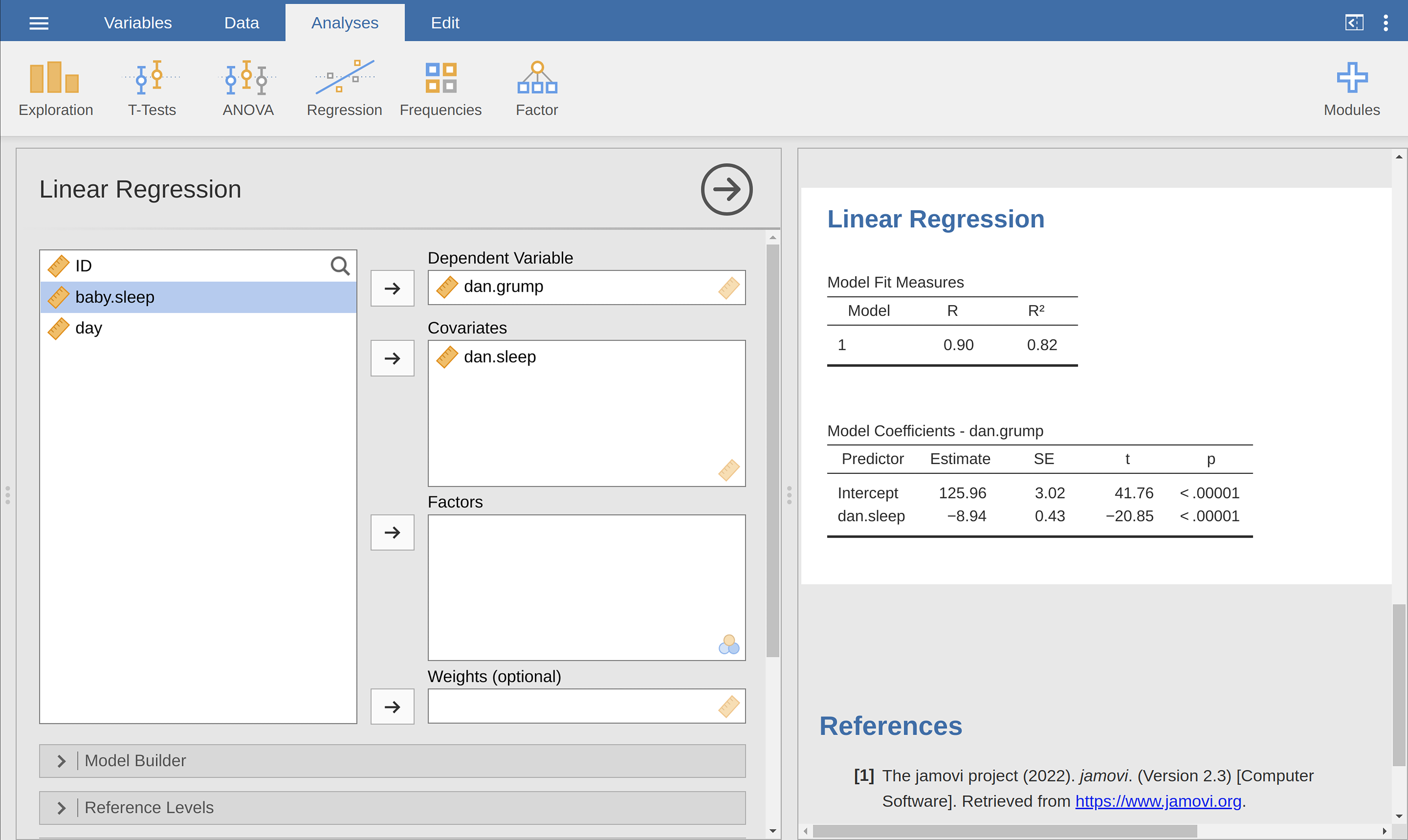
Fig. 136 jamovi screenshot showing a simple linear regression analysis

To run my linear regression, open up the Regression → Linear Regression analysis in jamovi, using the parenthood data set. Then specify dani.grump as the Dependent Variable and dani.sleep as the variable entered in the Covariates box. This gives the results shown in Fig. 136, showing an intercept \(\hat{b}_0\) = 125.96 and the slope \(\hat{b}_1\) = -8.94. In other words, the best-fitting regression line that I plotted in Fig. 135 has this formula:

Ŷ_i = 125.96 + (-8.94 X_i)

Interpreting the estimated model

The most important thing to be able to understand is how to interpret these coefficients. Let us start with \(\hat{b}_1\), the slope. If we remember the definition of the slope, a regression coefficient of \(\hat{b}_1\) = -8.94 means that if I increase X_i by 1, then I am decreasing Y_i by 8.94. That is, each additional hour of sleep that I gain will improve my mood, reducing my grumpiness by 8.94 grumpiness points. What about the intercept? Well, since \(\hat{b}_0\) corresponds to “the expected value of Y_i when X_i equals 0”, it is pretty straightforward. It implies that if I get zero hours of sleep (X_i = 0) then my grumpiness will go off the scale, to an insane value of (Y_i = 125.96). Best to be avoided, I think.

---

[1]

However, it will help you to know that the solution to the estimation problem turns out to be \(\hat{b} = (\mathbf{X} ^ \prime\mathbf{X}) ^ {-1} \mathbf{X} ^ \prime y\), where \(\hat{b}\) is a vector containing the estimated regression coefficients, X is the “design matrix” that contains the predictor variables (plus an additional column containing all ones; strictly X is a matrix of the regressors, but I have not discussed the distinction yet), and y is a vector containing the outcome variable. Since quite a few things in linear regression can be written in linear algebra terms, you will see a bunch of footnotes like this one in this chapter. If you can follow the maths in them, great. If not, ignore it.