Auteur de la section : Danielle J. Navarro and David R. Foxcroft
What is a linear regression model?
Stripped to its bare essentials, linear regression models are basically a
fancier version of the Pearson correlation (section Correlations),
but they are much more powerful tools. We will return to the parenthood data
set that we were using to illustrate how correlations work. Recall that, in
this data set we were trying to find out why Danielle is so very grumpy all the
time and our working hypothesis was that I am not getting enough sleep. We drew
some scatterplots to help us examine the relationship between the amount of
sleep I get and my grumpiness the following day, as in Fig. 132, and
as we saw previously this corresponds to a correlation of r = -0.90, but what
we find ourselves secretly imagining is something that looks closer to
Fig. 134 (a). That is, we mentally draw a straight line through the
middle of the data. In statistics, this line that we are drawing is called a
regression line. Notice that, since we are not idiots, the regression line
goes through the middle of the data. We do not find ourselves imagining anything
like the rather silly plot shown in Fig. 134 (b).
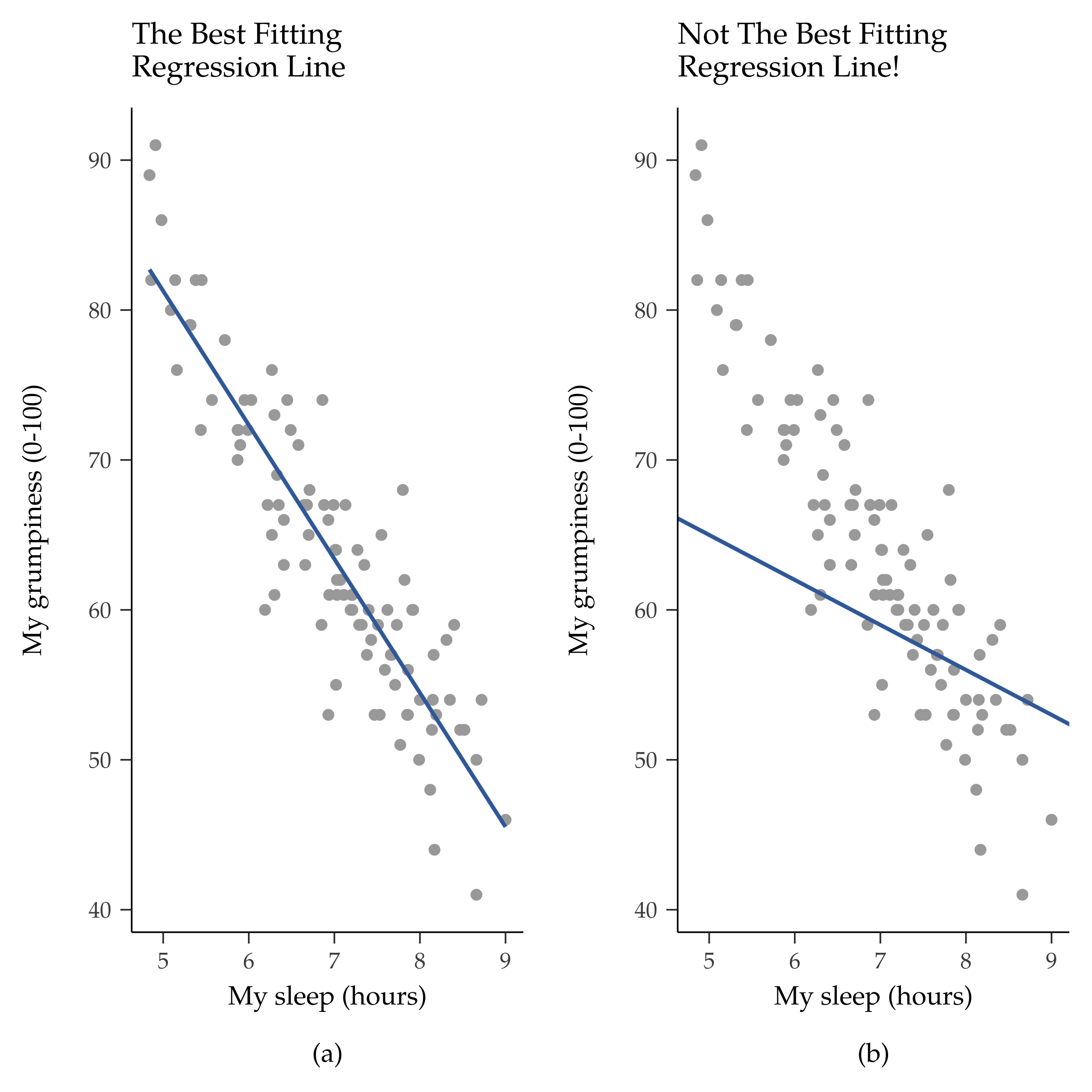
Fig. 134 Panel (a) shows the scatterplot of dani.sleep and dani.grump from
Fig. 132 with the best fitting regression line drawn over the top.
Not surprisingly, the line goes through the middle of the data. In contrast,
panel (b) shows the same data, but with a very poor choice of regression
line drawn over the top.
This is not highly surprising. The line that I have drawn in Fig. 134 (panel b) does not “fit” the data very well, so it does not make a lot of sense to propose it as a way of summarising the data, right? This is a very simple observation to make, but it turns out to be very powerful when we start trying to wrap just a little bit of maths around it. To do so, let us start with a refresher of some high school maths. The formula for a straight line is usually written like this:
The two variables are x and y, and we have two coefficients, a and b.[1] The coefficient a represents the y-intercept of the line, and coefficient b represents the slope of the line. The intercept is interpreted as “the value of y that you get when x = 0”. Similarly, a slope of b means that if you increase the x-value by 1 unit, then the y-value goes up by b units, and a negative slope means that the y-value would go down rather than up. If Y is the outcome variable (the DV) and X is the predictor variable (the IV), then the formula that describes our regression is written like this:
It looks like the same formula, but there is some extra frilly bits in this version. Let us make sure we understand them. Firstly, notice that I have written Xi and Yi rather than just plain old X and Y. This is because we want to remember that we are dealing with actual data. In this equation, Xi is the value of predictor variable for the ith observation (i.e., the number of hours of sleep that I got on day i of my little study), and Yi is the corresponding value of the outcome variable (i.e., my grumpiness on that day). And although I have not said so explicitly in the equation, what we are assuming is that this formula works for all observations in the data set (i.e., for all i). Secondly, notice that I wrote Ŷi and not Yi. This is because we want to make the distinction between the actual data Yi, and the estimate Ŷi (i.e., the prediction that our regression line is making). Thirdly, I changed the letters used to describe the coefficients from a and b to b0 and b1. That is just the way that statisticians like to refer to the coefficients in a regression model. I have no idea why they chose b, but that is what they did. In any case b0 always refers to the intercept term, and b1 refers to the slope.
Next, I can not help but notice that, regardless of whether we are talking about the good regression line or the bad one, the data do not fall perfectly on the line. Or, to say it another way, the data Yi are not identical to the predictions of the regression model Ŷi. Since statisticians love to attach letters, names and numbers to everything, let us refer to the difference between the model prediction and that actual data point as a residual, and we will refer to it as εi.[2] Written using mathematics, the residuals are defined as:
This, in turn, means that we can write down the complete linear regression model as: