Autor des Abschnitts: Danielle J. Navarro and David R. Foxcroft

Konfirmatorische Faktorenanalyse

So, our attempt to identify underlying latent factors using EFA with carefully selected questions from the personality item pool seemed to be pretty successful. The next step in our quest to develop a useful measure of personality is to check the latent factors we identified in the original EFA with a different sample. We want to see if the factors hold up, if we can confirm their existence with different data. This is a more rigorous check, as we will see. And it is called Confirmatory Factor Analysis (CFA) as we will, unsuprisingly, be seeking to confirm a pre-specificied latent factor structure.[1]

In CFA, instead of doing an analysis where we see how the data goes together in an exploratory sense, we instead impose a structure, like in Abb. 207, on the data and see how well the data fits our pre-specified structure. In this sense, we are undertaking a confirmatory analysis, to see how well a pre-specified model is confirmed by the observed data.

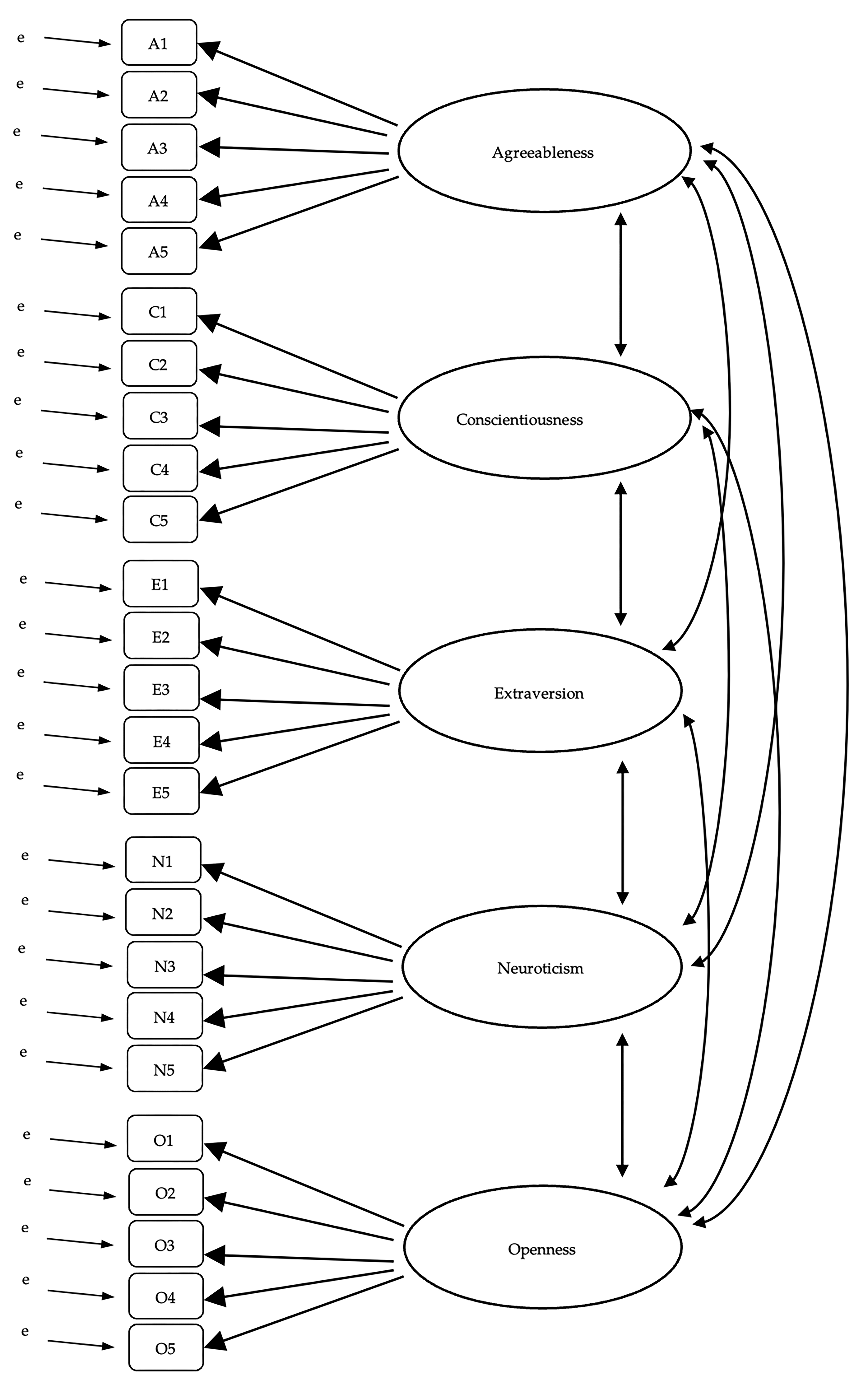
Abb. 207 Ursprüngliche Spezifizierung der latenten fünffaktoriellen Struktur für die Persönlichkeitsdaten zur Verwendung in einer CFA

A straightforward confirmatory factor analysis (CFA) of the personality items would therefore specify five latent factors as shown in Abb. 207, each measured by five observed variables. Each variable is a measure of an underlying latent factor. For example, A1 is predicted by the underlying latent factor Agreeableness. And because A1 is not a perfect measure of the Agreeableness factor, there is an error term, e, associated with it. In other words, e represents the variance in A1 that is not accounted for by the Agreeableness factor. This is sometimes called measurement error.

The next step is to consider whether the latent factors should be allowed to correlate in our model. As mentioned earlier, in the psychological and behavioural sciences constructs are often related to each other, and we also think that some of our personality factors may be correlated with each other. So, in our model, we should allow these latent factors to covary, as shown by the double-headed arrows in Abb. 207.

At the same time, we should consider whether there is any good, systematic, reason for some of the error terms to be correlated with each other. One reason for this might be that there is a shared methodological feature for particular sub-sets of the observed variables such that the observed variables might be correlated for methodological rather than substantive latent factor reasons. We will return to this possibility in a later section but, for now, there are no clear reasons that we can see that would justify correlating some of the error terms with each other.

Without any correlated error terms, the model we are testing to see how well it fits with our observed data is just as specified in Abb. 207. Only parameters that are included in the model are expected to be found in the data, so in CFA all other possible parameters (coefficients) are set to zero. So, if these other parameters are not zero (for example there may be a substantial loading from A1 onto the latent factor Extraversion in the observed data, but not in our model) then we may find a poor fit between our model and the observed data.

CFA in jamovi

To set this CFA analysis up in jamovi, we open up the bfi_sample2 data set, check that the 25 variables are coded as ordinal (or continuous ; it will not make any difference for this analysis), and perform a CFA using the following steps:

• Select Factor → Confirmatory Factor Analysis from the Analyses tab to open the options panel where you can determine the settings for the CFA (Abb. 208).

• Select the five A variables and transfer them into the Factors box and give them the label “Agreeableness”.

• Create a new Factor in the Factors box and label it “Conscientiousness”. Select the five C variables and transfer them into the Factors box under the “Conscientiousness” label.

• Create another new Factor in the Factors box and label it “Extraversion”. Select the five E variables and transfer them into the Factors box under the “Extraversion” label.

• Create another new Factor in the Factors box and label it “Neuroticism”. Select the five N variables and transfer them into the Factors box under the “Neuroticism” label.

• Create another new Factor in the Factors box and label it “Openness”. Select the five O variables and transfer them into the Factors box under the “Openness” label.

• Check other appropriate options, the defaults are OK for this initial work through, though you might want to check the Path diagram option under Plots to see jamovi produce a (fairly) similar diagram to our Abb. 207.

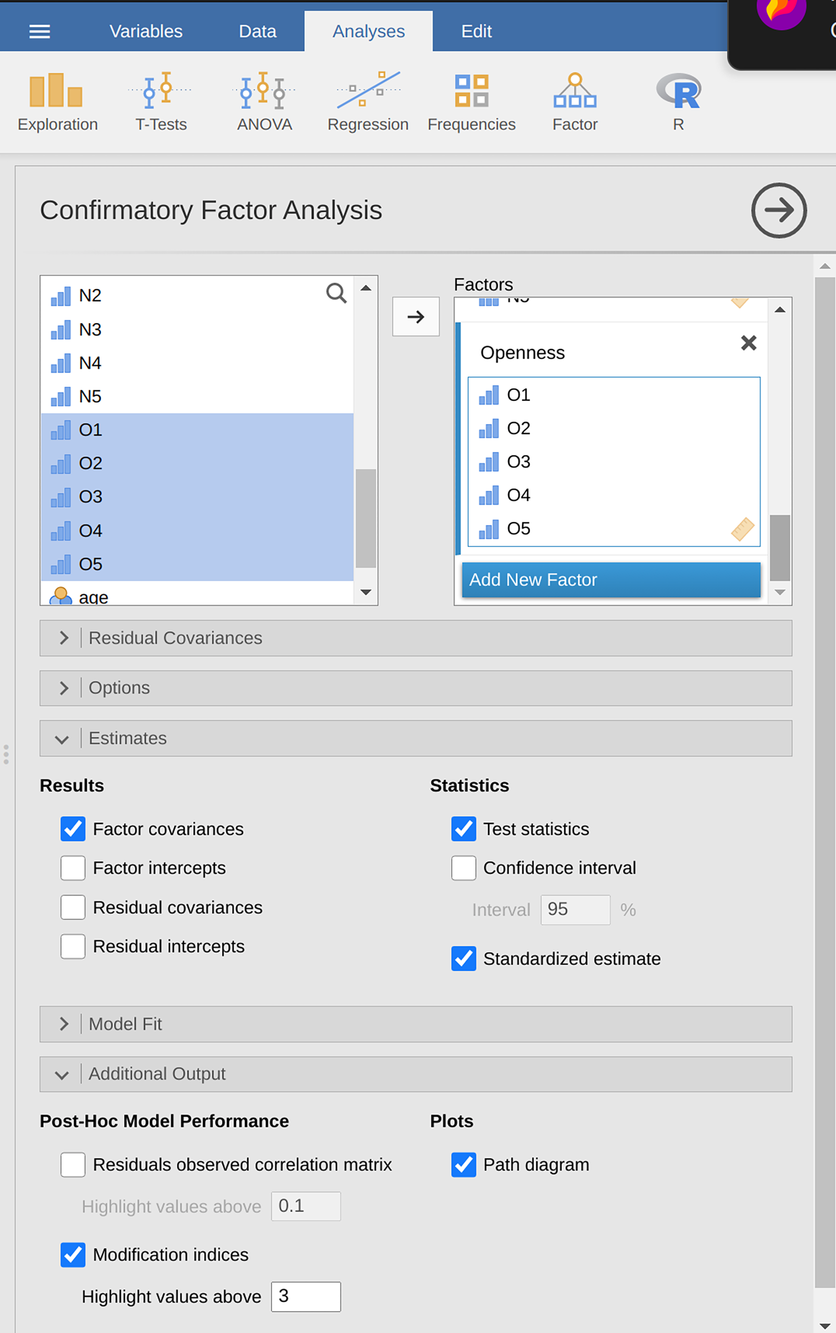
Abb. 208 Optionsfeld mit den Einstellungen zum Durchführen einer konfirmatorischen Faktorenanalyse (CFA) in jamovi

Once we have set up the analysis we can turn our attention to the jamovi results panel and see what is what. The first thing to look at is model fit (Abb. 209) as this tells us how good a fit our model is to the observed data. NB in our model only the pre-specified covariances are estimated, including the factor correlations by default. Everything else is set to zero.

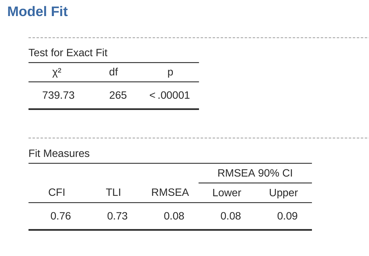
Abb. 209 Tabelle mit den Model Fit-Ergebnissen für das definierte CFA-Modell in jamovi

Es gibt mehrere Möglichkeiten, die Modellgüte zu bewerten. Die erste ist eine χ²-Statistik: Wenn sie klein ist, dann passt das Modell gut zu den Daten. Die hierbei verwendete χ²-Statistik ist jedoch ziemlich anfällig gegenüber dem Stichprobenumfang: Bei einer großen Stichprobe ergibt sich selbst bei einer ausreichend guten Anpassung zwischen dem Modell und den Daten fast immer ein großer und signifikanter (p < 0,05) χ²-Wert.

Wir brauchen also andere Methoden zur Bewertung der Modellgüte. jamovi bietet standardmäßig mehrere an. Dies sind der Comparative Fit Index (CFI), der Tucker-Lewis-Index (TLI) und der Root Mean Square Error of Approximation (RMSEA) zusammen mit dem 90%-Konfidenzintervall für den RMSEA. Einige nützliche Faustregeln besagen, dass eine zufriedenstellende Modellgüte bei CFI > 0,9, TLI > 0,9 und RMSEA von etwa 0,05 bis 0,08 gegeben ist. Eine gute Anpassung erfordert CFI > 0,95, TLI > 0,95 und RMSEA und oberer CI für RMSEA < 0,05.

So, looking at Abb. 209, we can see that the χ²-value is large and highly significant. Our sample size is not too large, so this possibly indicates a poor fit. The CFI is 0.762 and the TLI is 0.731, indicating poor fit between the model and the data. The RMSEA is 0.085 with a 90% confidence interval from 0.077 to 0.092, again this does not indicate a good fit.

Ziemlich enttäuschend, aber vielleicht nicht allzu überraschend, wenn man bedenkt, dass in der früheren EFA, die wir mit einem ähnlichen Datensatz durchgeführt haben (Abschnitt Explorative Faktorenanalyse), nur etwa die Hälfte der Varianz in den Daten durch das Fünf-Faktoren-Modell aufgeklärt werden konnte.

Let us go on to look at the factor loadings and the factor covariance estimates, shown in Abb. 210 and Abb. 211. The Z-statistic and p-value for each of these parameters indicates they make a reasonable contribution to the model (i.e., they are not zero) so there does not appear to be any reason to remove any of the specified variable-factor paths, or factor-factor correlations from the model. Often the standardized estimates are easier to interpret, and these can be specified under the Estimates option. These tables can usefully be incorporated into a written report or scientific article.

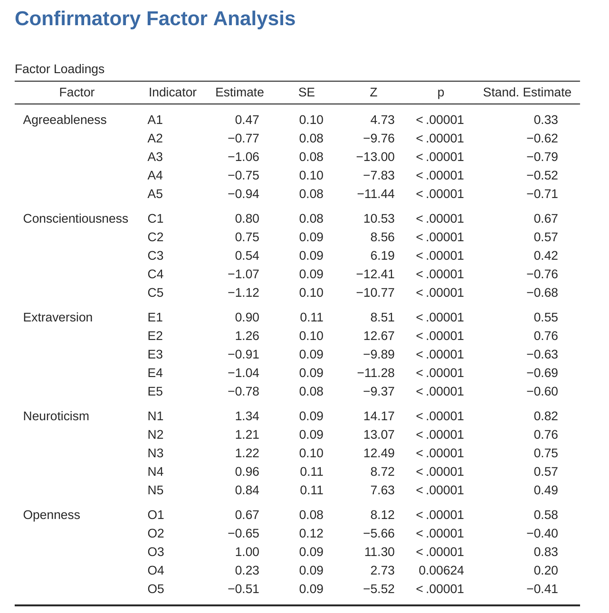
Abb. 210 Tabelle mit Factor Loadings für das definierte CFA-Modell in jamovi

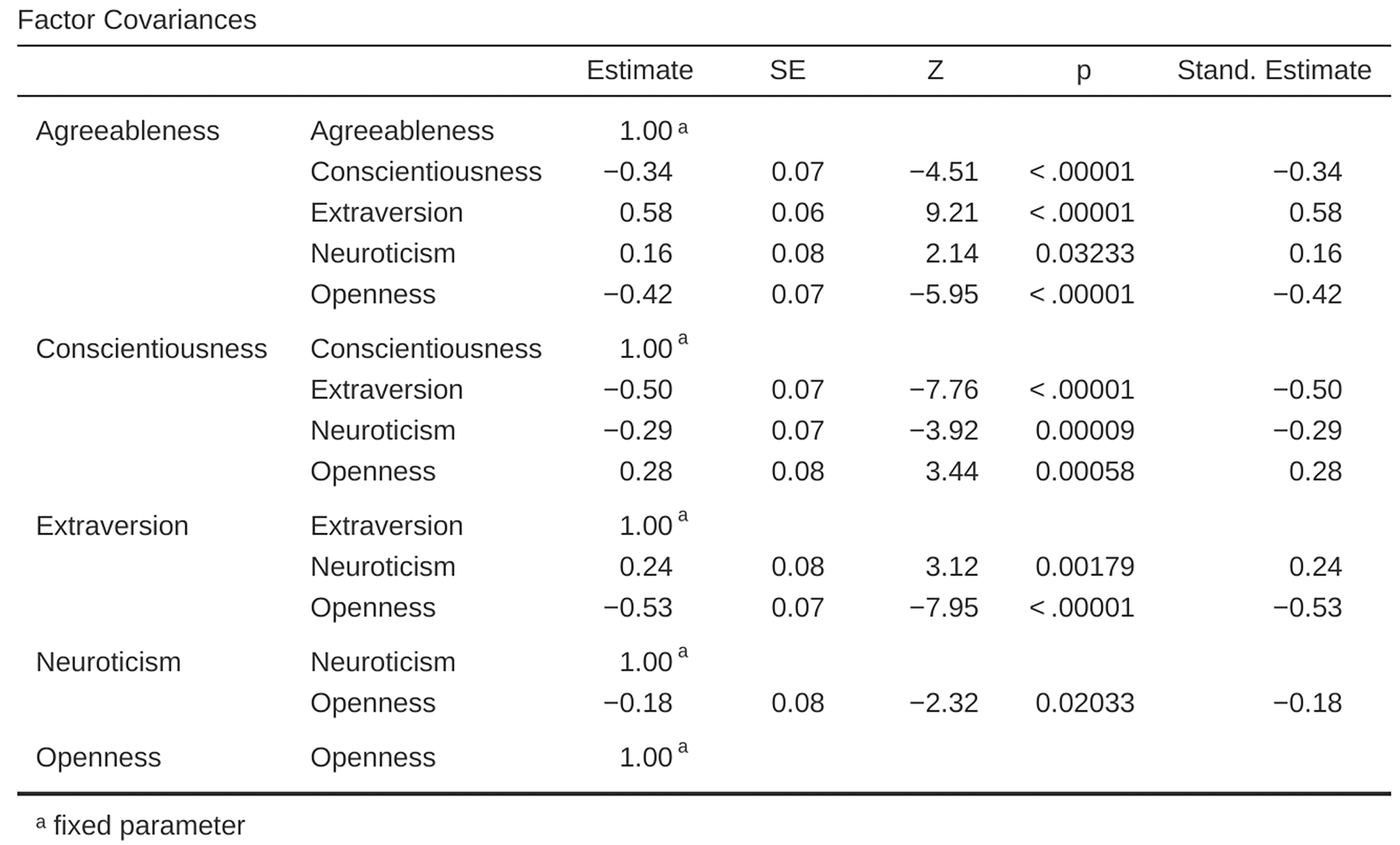
Abb. 211 Tabelle mit den Factor Covariances für das definierte CFA-Modell in jamovi

How could we improve the model? One option is to go back a few stages and think again about the items / measures we are using and how they might be improved or changed. Another option is to make some post-hoc tweaks to the model to improve the fit. One way of doing this is to use Modification indices, specified as an Additional Output option in jamovi (see Abb. 212).

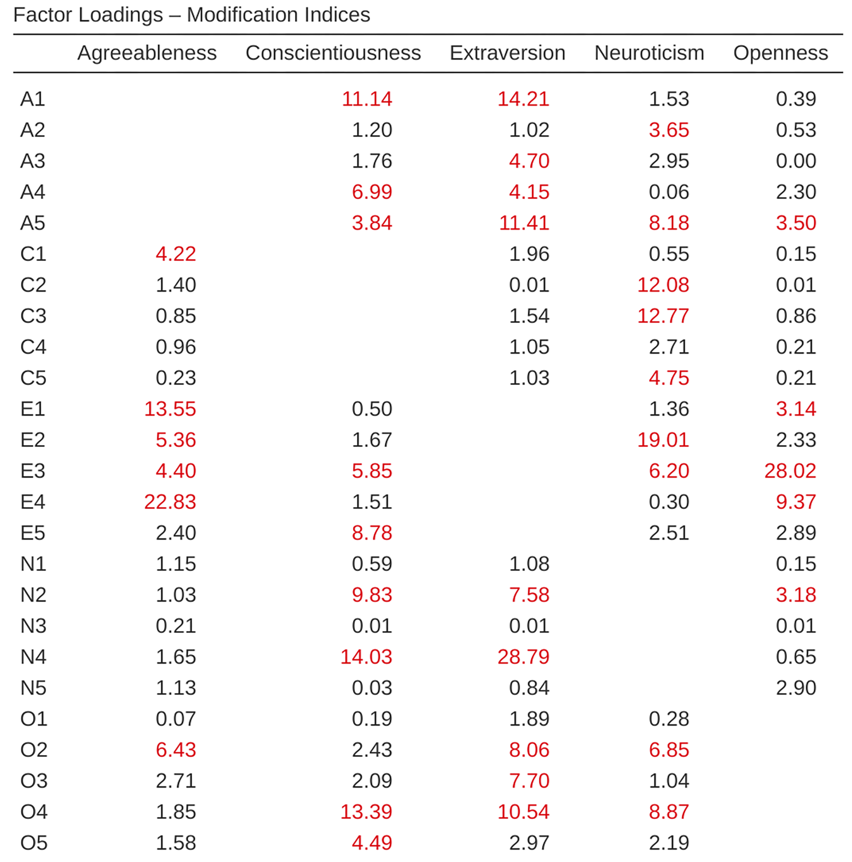
Abb. 212 Tabelle mit den Factor Loadings Modification Indices für das definierte CFA-Modell in jamovi

What we are looking for is the highest modification index (MI) value. We would then judge whether it makes sense to add that additional term into the model, using a post-hoc rationalisation. For example, we can see in Abb. 212 that the largest MI for the factor loadings that are not already in the model is a value of 28.786 for the loading of N4 (“Often feel blue”) onto the latent factor Extraversion. This indicates that if we add this path into the model then the χ²-value will reduce by around the same amount.

But in our model adding this path arguably does not really make any theoretical or methodological sense, so it is not a good idea (unless you can come up with a persuasive argument that “Often feel blue” measures both Neuroticism and Extraversion). I can not think of a good reason. But, for the sake of argument, let us pretend it does make some sense and add this path into the model. Go back to the CFA analysis window (see Abb. 208) and add N4 into the Extraversion factor. The results of the CFA will now change (not shown); the χ²-value has come down to around 709 (a drop of around 30, roughly similar to the size of the MI) and the other fit indices have also improved, though only a bit. But it is not enough: it is still not a good fitting model.

Wenn Sie unter Verwendung der MI-Werte neue Parameter zu einem Modell hinzufügen, sollten Sie die MI-Tabellen nach jeder neuen Hinzufügung erneut überprüfen, da die MI-Werte jedes Mal aktualisiert werden.

There is also a Table of Residual Covariances Modification Indices produced by jamovi (Abb. 213). In other words, a table showing which correlated errors, if added to the model, would improve the model fit the most. It is a good idea to look across both MI tables at the same time, spot the largest MI, think about whether the addition of the suggested parameter can be reasonably justified and, if it can, add it to the model. And then you can start again looking for the biggest MI in the re-calculated results.

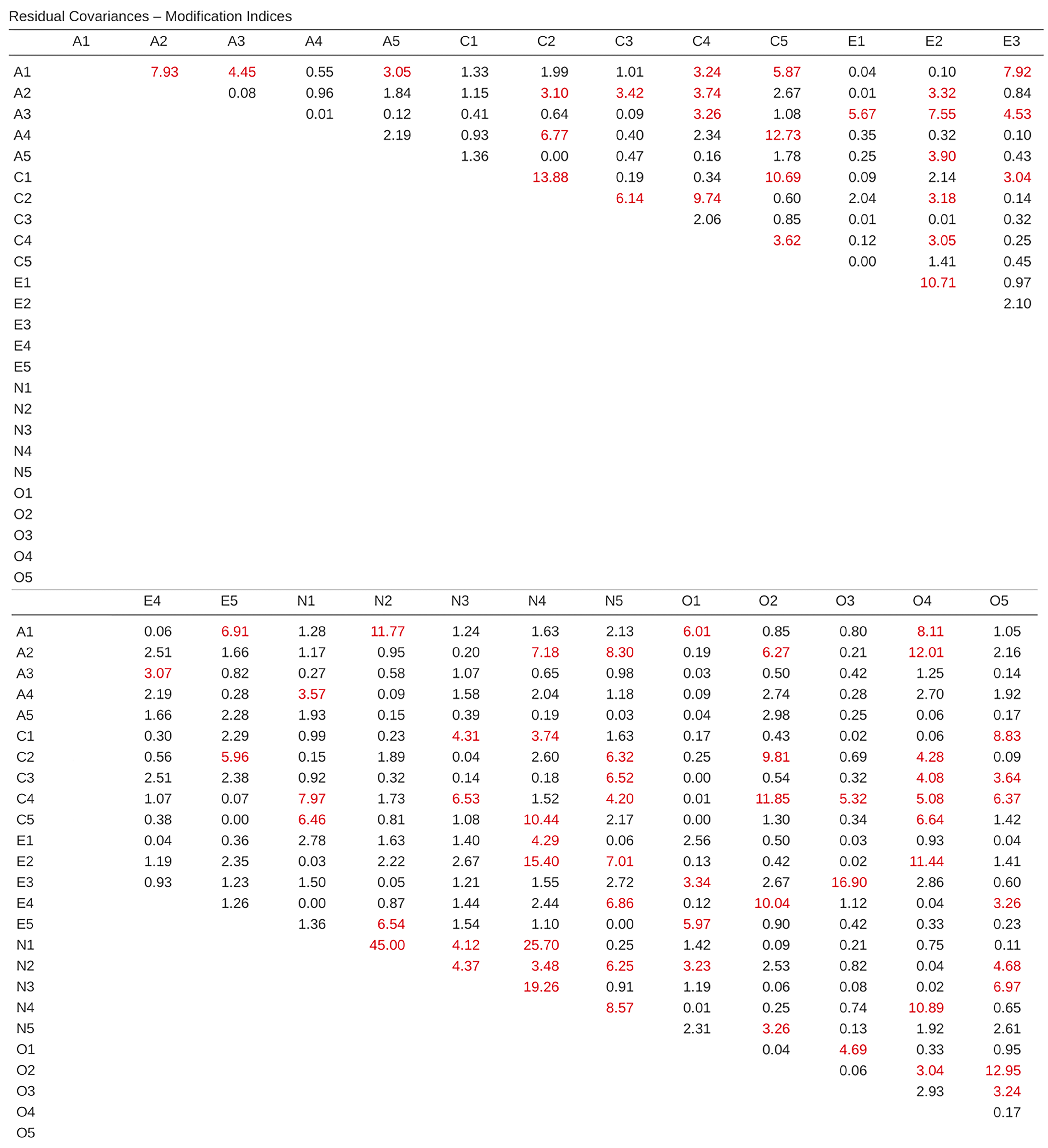
Abb. 213 Tabelle mit den Residual Covariances Modification Indices für das definierte CFA-Modell in jamovi

You can keep going this way for as long as you like, adding parameters to the model based on the largest MI, and eventually you will achieve a satisfactory fit. But there will also be a strong possibility that in doing this you will have created a monster! A model that is ugly and deformed and does not have any theoretical sense or purity. In other words, be very careful!

So far, we have checked out the factor structure obtained in the EFA using a second sample and CFA. Unfortunately, we did not find that the factor structure from the EFA was confirmed in the CFA, so it is back to the drawing board as far as the development of this personality scale goes.

Während es manchmal gute Gründe dafür gibt, dass Residuen kovariieren (oder korrelieren) dürfen, gab es keine solche vertretbaren Gründe die CFA für das von uns definierte Modell mit Hilfe von Modifikationsindizes durch das Einbeziehen zusätzlichen Faktorladungen oder Residualkovarianzen zu „optimieren“. Lassen Sie uns trotzdem besprechen, wie man die Ergebnisse einer CFA (bei einem besser angepassten Modell) berichten würde.

Berichten einer CFA

Es gibt keine formale Standardmethode für die Erstellung eines CFA, und die Beispiele variieren je nach Disziplin und Forscher. Dennoch gibt es einige Standardinformationen, die Sie in Ihren Bericht aufnehmen sollten:

1. Eine theoretische und empirische Begründung für das hypothetische Modell.

2. A complete description of how the model was specified (e.g., the indicator variables for each latent factor, covariances between latent variables, and any correlations between error terms). A path diagram, like the one in Abb. 207 would be good to include.

3. A description of the sample (e.g., demographic information, sample size, sampling method).

4. Eine Beschreibung der Art der verwendeten Daten (z. B. nominal , kontinuierlich ) sowie Deskriptivstatistik für diese Variablen.

5. Welche Voraussetzungen geprüft und welche Schätzmethode verwendet wurde.

6. Eine Beschreibung von fehlenden Werten und wie diese behandelt wurden.

7. Die für die Anpassung des Modells verwendete Statistiksoftware (inkl. der Versionsnummer).

8. Maße und Kriterien zur Beurteilung der Modellgüte.

9. Alle Änderungen, die am ursprünglichen Modell aufgrund von Modellanpassungs- oder Änderungsindizes vorgenommen wurden.

10. Alle Parameterschätzungen (d.h. Faktorladungen, Fehlervarianzen, latente (Ko-)Varianzen) sowie ihre Standardfehler, am besten in einer Tabelle.

---

[1]

Nebenbei bemerkt: Da wir aufgrund unserer anfänglichen „mutmaßlichen“ Faktoren eine ziemlich genaue Vorstellung unseres erwarteten Modells (bzw. unserer Faktorstruktur) hatten, hätten wir auch direkt zur CFA übergehen und den EFA-Schritt überspringen können. Ob Sie die EFA verwenden und dann zur CFA übergehen oder ob Sie direkt zur CFA übergehen, ist eine Frage der Einschätzung und des Vertrauens, das Sie in Ihr ursprüngliches Modell haben (in Bezug auf die Anzahl der Faktoren und Variablen). In den ersten Schritten während der Entwicklung von Skalen oder der Identifizierung der zugrundeliegenden latenten Konstrukte neigen Forscher dazu, die EFA zu verwenden. Später, wenn sie sich einer endgültigen Skala nähern oder wenn sie eine etablierte Skala bei einer neuen Stichprobe überprüfen wollen, ist die CFA die Option der Wahl.