Autor des Abschnitts: Danielle J. Navarro and David R. Foxcroft

Explorative Faktorenanalyse

Die Explorative Faktorenanalyse (EFA) ist ein statistisches Verfahren zur Aufdeckung verborgener latenter Faktoren, die aus den beobachteten Daten abgeleitet werden. Mit dieser Technik wird berechnet, inwieweit ein Satz gemessener Variablen, z. B. V1, V2, V3, V4 und V5, einen möglichen zugrunde liegenden latenten Faktor repräsentiert. Dieser latente Faktor kann nicht durch eine einzige beobachtete Variable gemessen werden, sondern manifestiert sich in den Beziehungen, die er in einer Reihe von beobachteten Variablen verursacht.

In Abb. 196 each observed variable V is “caused” to some extent by the underlying latent factor (F), depicted by the coefficients b1 to b5 (also called factor loadings). Each observed variable also has an associated error term, e1 to e5. Each error term is the variance in the associated observed variable, V_i, that is unexplained by the underlying latent factor.

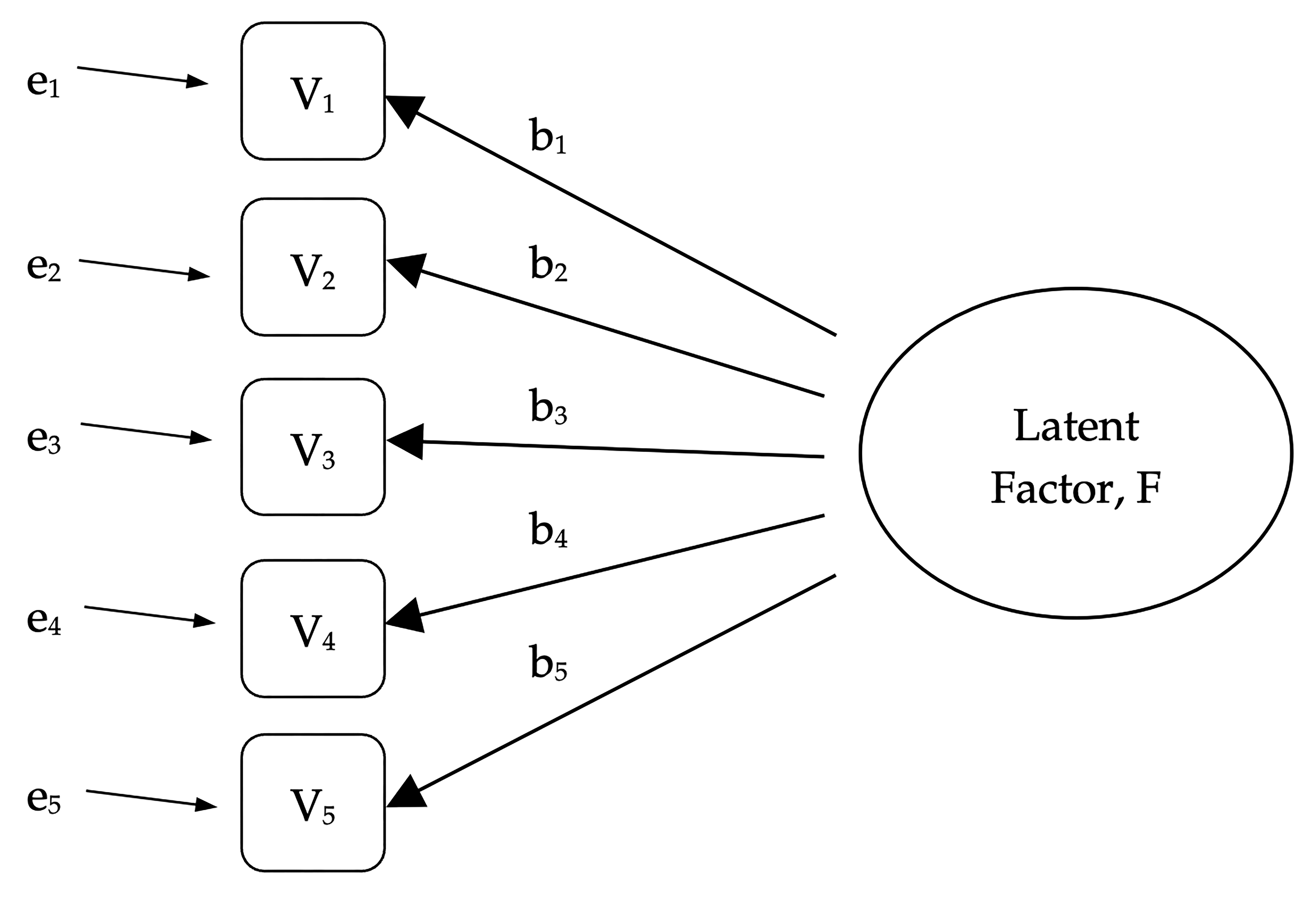
Abb. 196 Latenter Faktor, welcher der Beziehung zwischen beobachteten Variablen zugrunde liegt

In Psychology, latent factors represent psychological phenomena or constructs that are difficult to directly observe or measure. For example, personality, or intelligence, or thinking style. In the example in Abb. 196, we may have asked people five specific questions about their behaviour or attitudes, and from that we are able to get a picture about a personality construct called, for example, extraversion. A different set of specific questions may give us a picture about an individual’s introversion, or their conscientiousness.

Here is another example: we may not be able to directly measure statistics anxiety, but we can measure whether statistics anxiety is high or low with a set of questions in a questionnaire. For example, “Q1: Doing the assignment for a statistics course”, “Q2: Trying to understand the statistics described in a journal article”, and “Q3: Asking the lecturer for help in understanding something from the course”, etc., each rated from low anxiety to high anxiety. People with high statistics anxiety will tend to give similarly high responses on these observed variables because of their high statistics anxiety. Likewise, people with low statistics anxiety will give similar low responses to these variables because of their low statistics anxiety.

In Exploratory Factor Analysis (EFA), we are essentially exploring the correlations between observed variables to uncover any interesting, important underlying (latent) factors that are identified when observed variables covary. We can use statistical software to estimate any latent factors and to identify which of our variables have a high loading[1] (e.g., loading > 0.5) on each factor, suggesting they are a useful measure, or indicator, of the latent factor. Part of this process includes a step called rotation, which to be honest is a pretty weird idea but luckily we do not have to worry about understanding it; we just need to know that it is helpful because it makes the pattern of loadings on different factors much clearer. As such, rotation helps with seeing more clearly which variables are linked substantively to each factor. We also need to decide how many factors are reasonable given our data, and helpful in this regard is something called Eigen values. We will come back to this in a moment, after we have covered some of the main assumptions of EFA.

Überprüfen der Voraussetzungen

There are a couple of assumptions that need to be checked as part of the analysis. The first assumption is sphericity, which essentially checks that the variables in your data set are correlated with each other to the extent that they can potentially be summarised with a smaller set of factors. Bartlett’s test for sphericity checks whether the observed correlation matrix diverges significantly from a zero (or null) correlation matrix. So, if Bartlett’s test is significant (p < 0.05), this indicates that the observed correlation matrix is significantly divergent from the null, and is therefore suitable for EFA.

Die zweite Annahme ist Stichprobenangemessenheit und wird mit dem Kaiser-Meyer-Olkin (KMO)-Maß der Stichprobenangemessenheit (MSA) überprüft. Der KMO-Index ist ein Maß für den Anteil der Varianz unter den beobachteten Variablen, bei dem es sich um gemeinsame Varianz handelt. Mit Hilfe von partiellen Korrelationen wird geprüft, ob es Faktoren gibt, die Ladungen auf nur zwei Items aufweisen. Dieser Fall ist gegeben, wenn die Korrelation zweier Variablen deutlich größer ist, als die partielle Korrelation dieser zwei Variablen, bei der für den Einfluss aller andren Variablen kontrolliert wird. Es ist selten, wenn überhaupt, erwünscht, dass die EFA eine Vielzahl von Faktoren ergibt, die jeweils nur auf zwei Items laden. Ist der KMO-Index hoch (≈ 1), lassen sich Faktoren gut mittels einer EFA extrahieren, während die Daten bei einem niedrigen KMO-Wert (≈ 0) nicht für eine EFA geeignet ist. KMO-Werte unter 0,5 bedeuten, dass die Daten nicht für eine EFA geeignet sind, und ein KMO-Wert von 0,6 sollte vorliegen, bevor die EFA als geeignet angesehen wird. Werte zwischen 0,6 und 0,7 gelten als angemessen, Werte zwischen 0,7 und 0,9 als gut und Werte zwischen 0,9 und 1,0 als ausgezeichnet.

Wozu ist die EFA gut?

If the EFA has provided a good solution (i.e., a good factor model), then we need to decide what to do with our shiny new factors. Researchers often use EFA during psychometric scale development. They will develop a pool of questionnaire items that they think relate to one or more psychological constructs, use EFA to see which items “go together” as latent factors, and then they will assess whether some items should be removed because they do not usefully or distinctly measure one of the latent factors.[2]

In Verbindung mit diesem Ansatz besteht ein weiteres Ergebnis einer EFA darin, die Variablen, die auf unterschiedlichen Faktoren laden, jeweils zu einem Faktorwert zu kombinieren, der manchmal auch als Skalenwert bezeichnet wird. Es gibt zwei Optionen für die Kombination von Variablen zu einem Skalenwert:

• Erstellen Sie eine neue Variable mit einer nach den Faktorladungen gewichteten Antwort (score) für jedes Item, das zum Faktor beiträgt.

• Erstellen Sie eine neue Variable auf der Grundlage der einem Faktor zugeordneten Items, aber gewichten Sie sie diese gleich.

In the first option each item’s contribution to the combined score depends on how strongly it relates to the factor. In the second option we typically just average across all the items that contribute substantively to a factor to create the combined scale score variable. Which to choose is a matter of preference, though a disadvantage with the first option is that loadings can vary quite a bit from sample to sample, and in behavioural and health sciences we are often interested in developing and using composite questionnaire scale scores across different studies and different samples. In which case it is reasonable to use a composite measure that is based on the substantive items contributing equally rather than weighting by sample specific loadings from a different sample. In any case, understanding a combined variable measure as an average of items is simpler and more intuitive than using a sample specific optimally-weighted combination. But let us not get ahead of ourselves; what we should really focus on now is how to do an EFA in jamovi.

EFA in jamovi

First, we need some data. Twenty-five personality self-report items (see Tab. 18) taken from the International Personality Item Pool (https://ipip.ori.org) were included as part of the Synthetic Aperture Personality Assessment web-based personality assessment (SAPA; https://sapa-project.org) project. The 25 items are short phrases that one should respond to by indicating how accurately the statement describes one’s typical behaviour or attitudes. The items are organized by five putative factors: Agreeableness, Conscientiousness, Extraversion, Neuroticism, and Openness.

Tab. 18 Fünfundzwanzig beobachtete Variablen-Items, geordnet nach fünf mutmaßlichen Persönlichkeitsdimensionen im Datensatz bfi_sample. Wenn in der zweiten Spalte ein R steht, ist das Item invertiert.

Name		Frage / Item
A1	R	Gleichgültig gegenüber den Gefühlen anderer.
A2		Sich nach dem Wohlbefinden anderer erkundigen.
A3		Wissen, wie Sie andere trösten können.
A4		Kinder lieben.
A5		Dafür sorgen, dass sich die Menschen wohlfühlen.
C1		Anspruchsvoll in meiner Arbeit sein.
C2		Fortfahren, bis alles perfekt ist.
C3		Dinge entsprechend einem Plan erledigen.
C4	R	Dinge nur mit halber Kraft erledigen.
C5	R	Zeit verschwenden.
E1	R	Nicht viel reden.
E2	R	Es schwierig finden, auf andere zuzugehen.
E3		Wissen, wie man Menschen fesselt.
E4		Leicht Freunde finden.
E5		Verantwortung übernehmen.
N1		Leicht wütend werden.
N2		Leicht gereizt werden.
N3		Häufige Stimmungsschwankungen.
N4		Sich oft traurig fühlen.
N5		Leicht in Panik geraten.
O1		Voller Ideen stecken.
O2	R	Schwierigen Lesestoff vermeiden.
O3		Gespräche auf ein höheres Niveau bringen.
O4		Zeit damit verbringen, über Dinge nachzudenken.
O5	R	Nicht tief in ein Thema eindringen.

Die Daten wurden mit Hilfe einer 6-stufigen Antwortskala erhoben:

1. Trifft überhaupt nicht zu

2. Trifft nicht zu

3. Trifft eher nicht zu

4. Trifft eher zu

5. Trifft zu

6. Trifft absolut zu.

Eine Stichprobe von N = 250 Antworten ist im Datensatz bfi_sample enthalten. Neben den Items gibt es drei weitere Spalten im Datensatz: ID (die Teilnehmer-ID, eine fünfstellige Zahl) sowie das Alter (age) und das Geschlecht (gender) der Befragten.

As researchers, we are interested in exploring the data to see whether there are some underlying latent factors that are measured reasonably well by the 25 observed variables in the bfi_sample data set. Open it up and check that the 25 variables are coded as continuous variables (technically they are ordinal though for EFA in jamovi it mostly does not matter, except if you decide to calculate weighted factor scores in which case continuous variables are needed). To perform an EFA in jamovi:

• Select Factor → Exploratory Factor Analysis from the Analyses tab to open the options panel where you can determine the settings for the EFA (Abb. 197).

• Wählen Sie die 25 Persönlichkeitsfragen aus und übertragen Sie diese in das Feld Variables.

• Check appropriate options, including Assumption Checks, but also Rotation under Method, Number of Factors to extract, and Additional Output options (see Abb. 197 for suggested options for this illustrative EFA, and please note that the Rotation under Method and Number of Factors extracted is typically adjusted by the researcher during the analysis to find the best result, as described below).

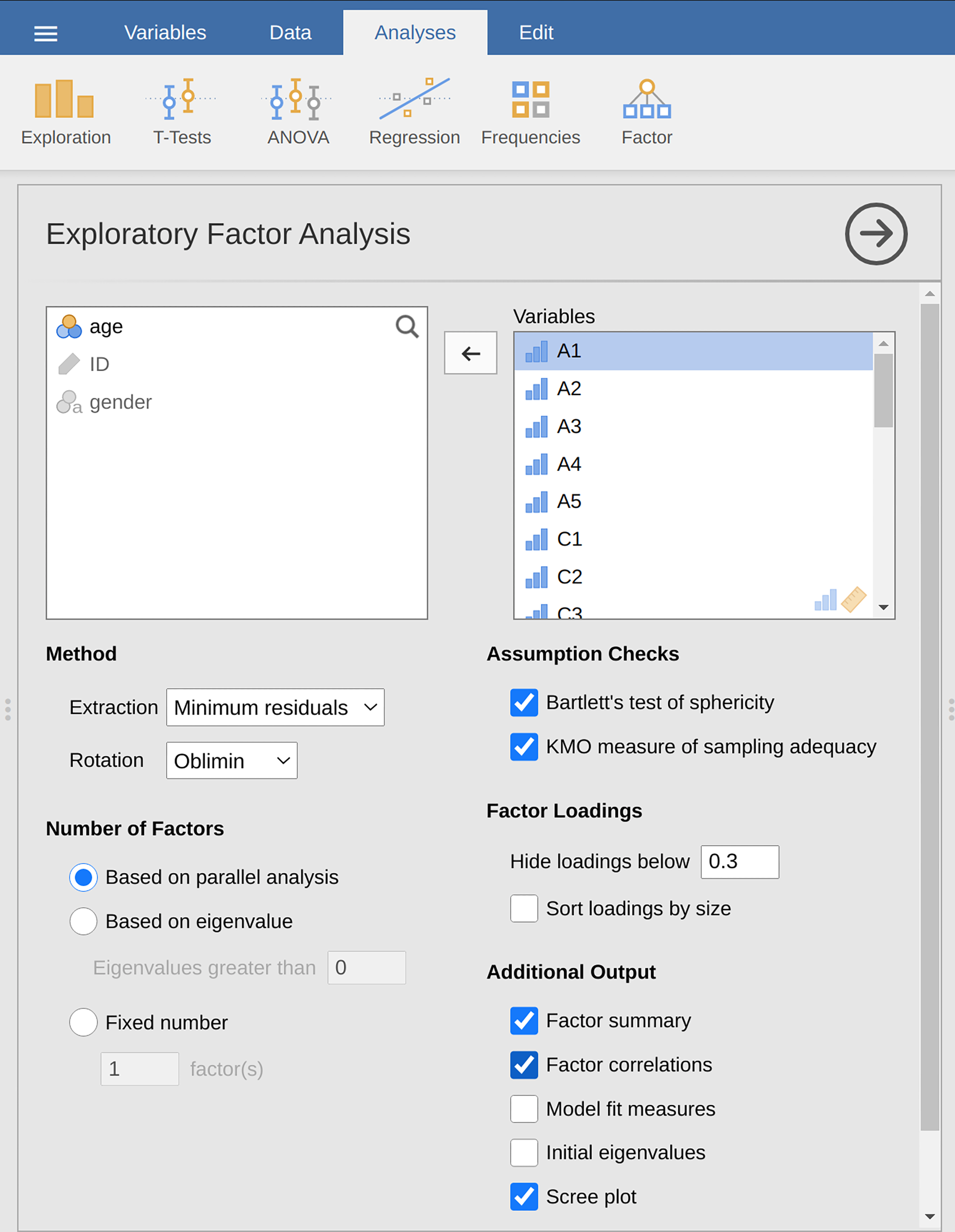
Abb. 197 Optionsfeld mit den Einstellungen zum Durchführen einer explorativen Faktorenanalyse (EFA) in jamovi

First, check the assumptions (Abb. 198). You can see that (1) Bartlett’s test of sphericity is significant, so this assumption is satisfied; and (2) the KMO measure of sampling adequacy (MSA) is 0.81 overall, suggesting good sampling adequacy. No problems here then!

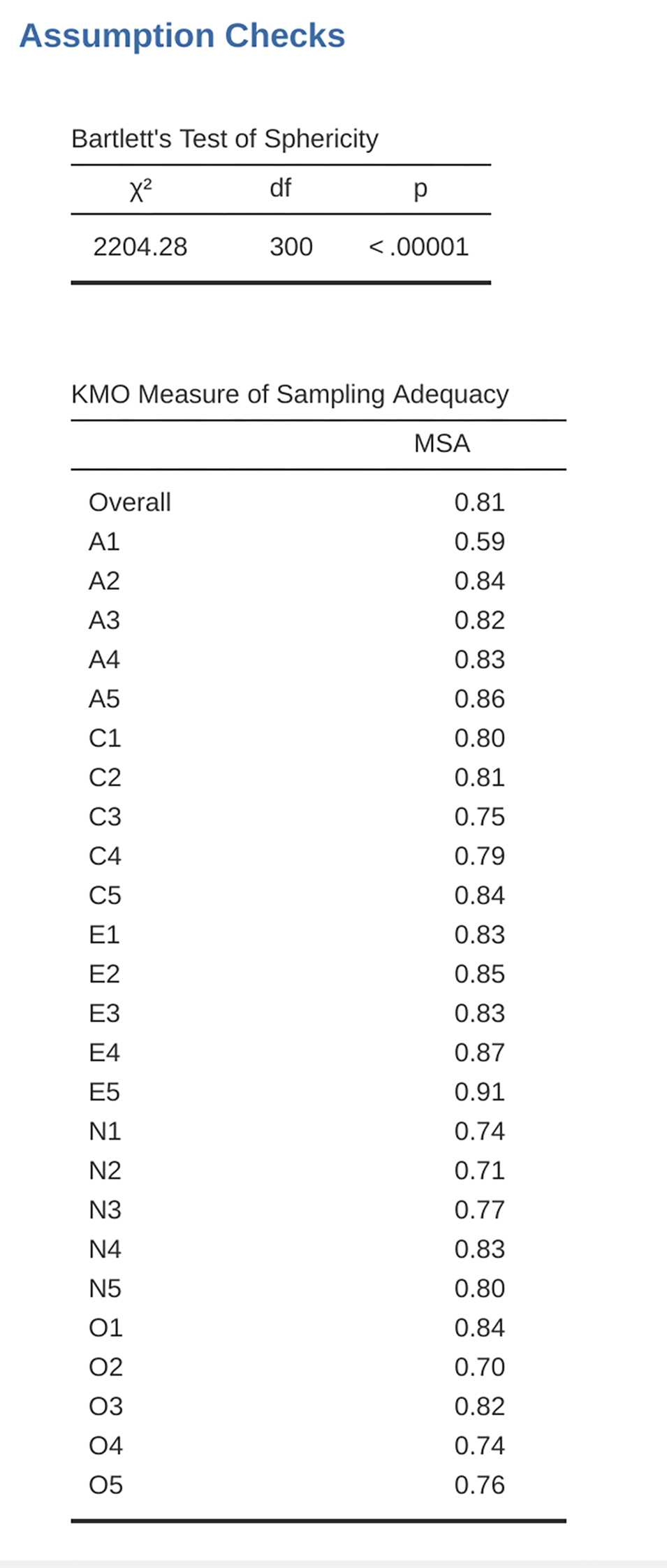
Abb. 198 Überprüfen der Voraussetzungen für eine EFA für die Daten des Persönlichkeitsfragebogens in jamovi

Als Nächstes ist zu prüfen, wie viele Faktoren verwendet (oder aus den Daten „extrahiert“) werden sollen. Es gibt drei verschiedene Ansätze:

• Eine Konvention ist es, alle Komponenten mit Eigenwerten größer als 1,[3] auszuwählen. Damit würden wir aus unseren Daten vier Faktoren extrahieren (probieren Sie es aus).

• Examination of the scree plot, as in Abb. 199, lets you identify the “point of inflection”. This is the point at which the slope of the scree curve clearly levels off, below the “elbow”. This would give us five factors with our data. Interpreting scree plots is a bit of an art: in Abb. 199 there is a noticeable step from five to seix factors, but in other scree plots you look at it will not be so clear cut.

• Mit Hilfe einer Technik der Parallelanalyse werden die aus den Daten erhaltenen Eigenwerte mit denen verglichen, die sich aus Zufallsdaten ergeben würden. Die Anzahl der extrahierten Faktoren ist die Anzahl der Eigenwerte, die größer sind als die, welche man mit Zufallsdaten erhalten würde.

Abb. 199 Scree-Plot der Persönlichkeitsdaten während der EFA in jamovi; nach Punkt 5 zeigt sich ein deutlicher Knick und eine Abflachung (der „Ellbogen“)

Der dritte Ansatz ist laut Fabrigar et al. (1999) eine gute Herangehensweise, obwohl Forscher in der Praxis dazu neigen, alle drei Ansätze zu betrachten und dann ein Urteil über die Anzahl der Faktoren zu fällen, die am einfachsten oder hilfreichsten zu interpretieren sind. Dies kann als „Sinnhaftigkeitskriterium“ verstanden werden, und die Forscher werden in der Regel neben der Lösung aus einem der oben genannten Ansätze auch Lösungen mit einer oder zwei Faktoren mehr oder weniger untersuchen. Sie entscheiden sich dann für die Lösung, die für sie am sinnvollsten ist.

At the same time, we should also consider the best way to rotate the final solution. There are two main approaches to rotation: orthogonal (e.g., Varimax) rotation forces the selected factors to be uncorrelated, whereas oblique (e.g., Oblimin) rotation allows the selected factors to be correlated. Dimensions of interest to psychologists and behavioural scientists are not often dimensions we would expect to be orthogonal, so oblique solutions are arguably more sensible.[4]

Practically, if in an oblique rotation the factors are found to be substantially correlated (positive or negative, and > 0.3), as in Abb. 200 where a correlation between two of the extracted factors is 0.31, then this would confirm our intuition to prefer oblique rotation. If the factors are, in fact, correlated, then an oblique rotation will produce a better estimate of the true factors and a better simple structure than will an orthogonal rotation. And, if the oblique rotation indicates that the factors have close to zero correlations between one another, then the researcher can go ahead and conduct an orthogonal rotation (which should then give about the same solution as the oblique rotation).

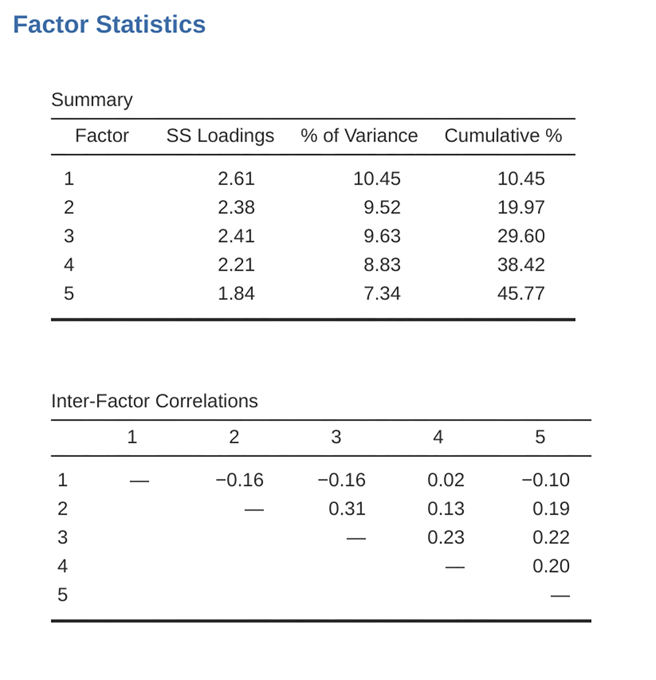
Abb. 200 Zusammenfassende Statistik der Faktoren und Korrelationen für eine EFA-Lösung mit fünf Faktoren in jamovi

On checking the correlation between the extracted factors at least one correlation was greater than 0.3 (Abb. 200), so an oblique (Oblimin) rotation of the five extracted factors is preferred. We can also see in Abb. 200 that the proportion of overall variance in the data that is accounted for by the five factors is 46%. Factor 1 accounts for around 10% of the variance, factors 2 to 4 around 9% each, and factor 5 just over 7%. This is not great; it would have been better if the overall solution accounted for a more substantive proportion of the variance in our data.

Seien Sie sich bewusst, dass Sie bei jeder EFA potenziell die gleiche Anzahl von Faktoren wie beobachtete Variablen haben können. Allerdings fügt jeder zusätzliche Faktor, den Sie einbeziehen, oft nur einen relativ kleinen Betrag an erklärter Varianz hinzu. Wenn die ersten paar Faktoren einen guten Teil der Varianz in den ursprünglichen 25 Variablen erklären, dann sind diese Faktoren eindeutig ein nützlicher, einfacher Ersatz für die 25 Variablen. Sie können den Rest weglassen, ohne dass zu viel von der ursprünglichen Varianz verloren geht (unerklärt bleibt). Wenn jedoch (zum Beispiel) 18 Faktoren erforderlich sind, um den größten Teil der Varianz in diesen 25 Variablen zu erklären, dann sollten Sie eher die ursprünglichen 25 Variablen verwenden.

Abb. 201 shows the factor loadings. That is, how the 25 different personality items load onto each of the five selected factors. We have hidden loadings less than 0.3 (set in the options shown in Abb. 197).

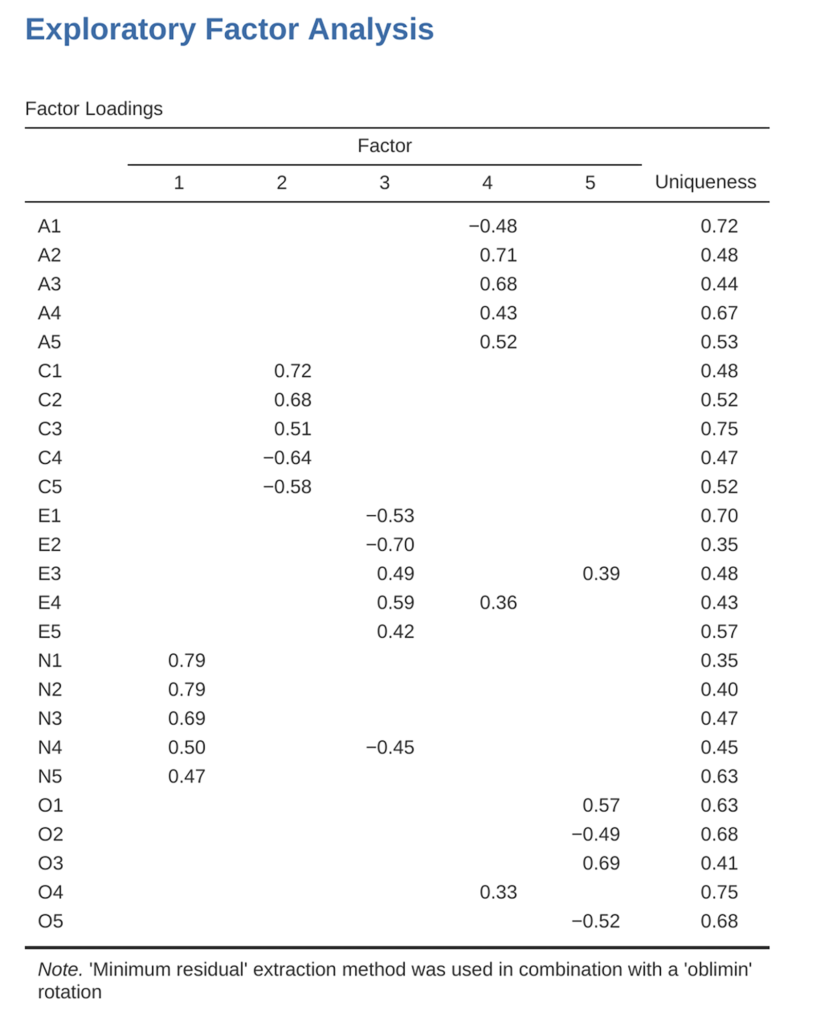
Abb. 201 Faktorladungen für eine EFA-Lösung mit fünf Faktoren in jamovi

For factors 1, 2, 3 and 4 the pattern of factor loadings closely matches the putative factors specified in Tab. 18. Phew! And factor 5 is pretty close, with four of the five observed variables that putatively measure “Openness” loading pretty well onto the factor. Variable O4 does not quite seem to fit though, as the factor solution in Abb. 201 suggests that it loads onto factor 4 (albeit with a relatively low loading) but not substantively onto factor 5.

The other thing to note is that those variables that were denoted as “R: reverse coding” in Tab. 18 are those that have negative factor loadings. Take a look at the items A1 (“Am indifferent to the feelings of others”) and A2 (“Inquire about others’ well-being”). We can see that a high score on A1 indicates low Agreeableness, whereas a high score on A2 (and all the other A-variables for that matter) indicates high Agreeableness. Therefore A1 will be negatively correlated with the other A-variables, and this is why it has a negative factor loading, as shown in Abb. 201.

We can also see in Abb. 201 the Uniqueness of each variable. Uniqueness is the proportion of variance that is “unique” to the variable and not explained by the factors.[5] For example, 72% of the variance in A1 is not explained by the factors in the five factor solution. In contrast, N1 has relatively low variance not accounted for by the factor solution (35%). Note that the greater the Uniqueness, the lower the relevance or contribution of the variable in the factor model.

To be honest, it is unusual to get such a neat solution in EFA. It is typically quite a bit more messy than this, and often interpreting the meaning of the factors is more challenging. It is not often that you have such a clearly delineated item pool. More often you will have a whole heap of observed variables that you think may be indicators of a few underlying latent factors, but you do not have such a strong sense of which variables are going to go where!

So, we seem to have a pretty good five factor solution, albeit accounting for a relatively low overall proportion of the observed variance. Let us assume we are happy with this solution and want to use our factors in further analysis. The straightforward option is to calculate an overall (average) score for each factor by adding together the score for each variable that loads substantively onto the factor and then dividing by the number of variables. For each person in our data set that would mean, for example for the Agreeableness factor, adding together A1 + A2 + A3 + A4 + A5, and then dividing by 5.[6] In essence, this means that the factor score we have calculated is based on equally weighted scores from each of the included variables. We can do this in jamovi in two steps:

1. Recode A1 into A1R by reverse scoring the values in the variable (i.e., 6 = 1; 5 = 2; 4 = 3; 3 = 4; 2 = 5; 1 = 6) using the jamovi transform variable function (see Abb. 202).

2. Compute a new variable, called Agreeableness, by calculating the mean of A1R, A2, A3, A4 and A5. Do this using the jamovi Compute command to create a new variable (see Abb. 203).

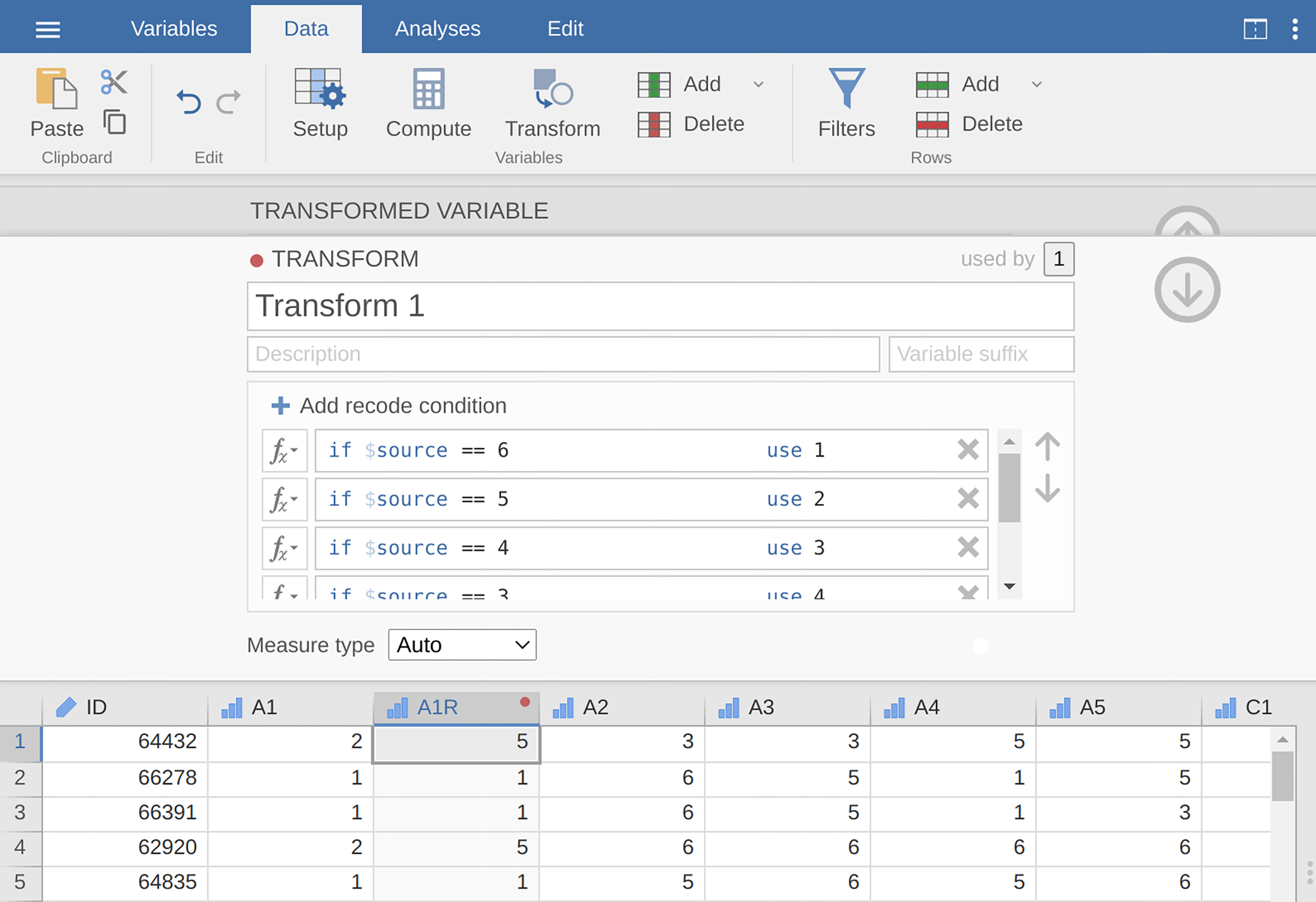
Abb. 202 Umkodierung der Variablen mit dem jamovi-Befehl Transform Variable

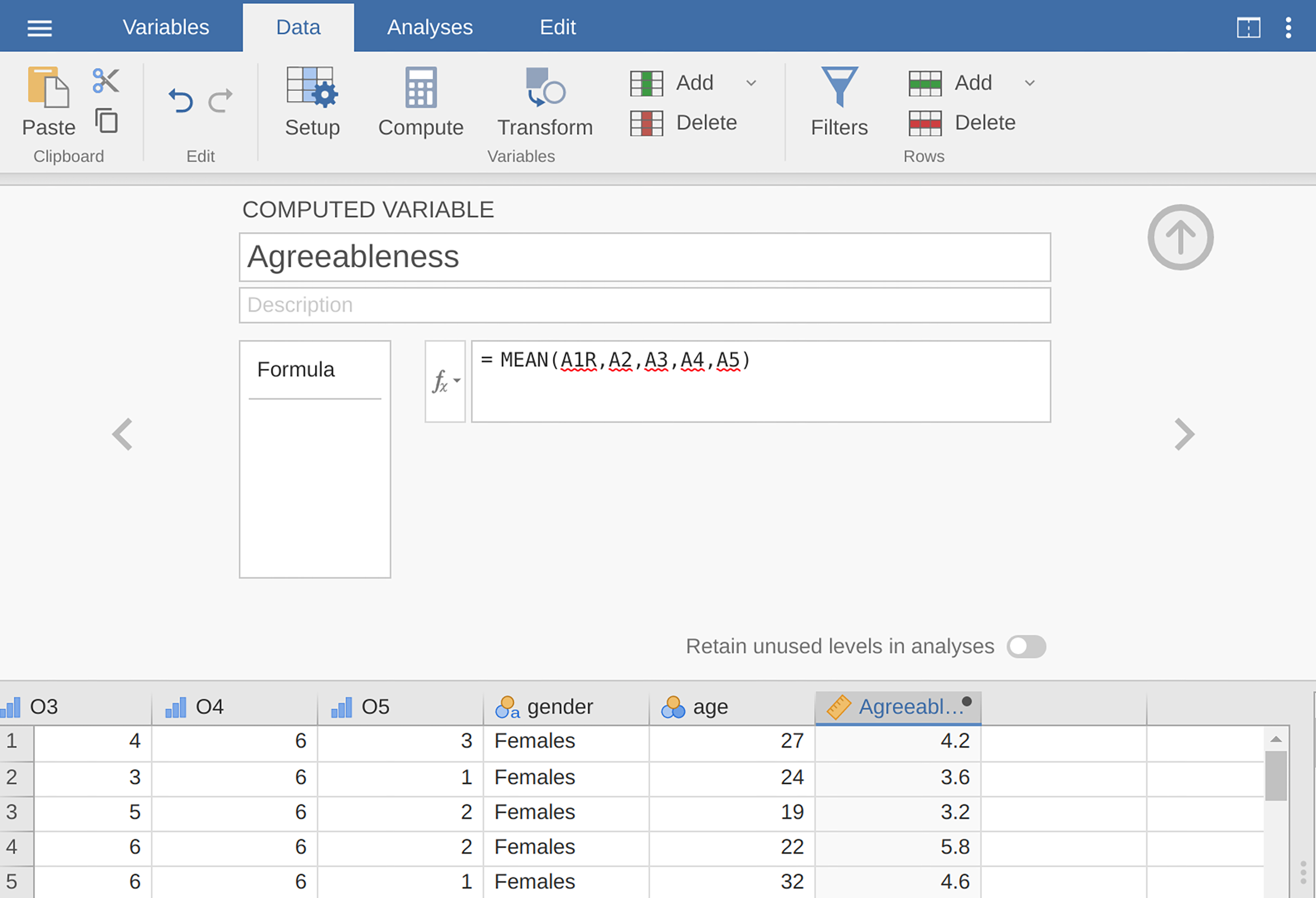
Abb. 203 Berechnung einer neuen Skalenwert-Variable unter Verwendung einer berechneten Variable in jamovi

Another option is to create an optimally-weighted factor score index. To do this, save the factor scores to the data set, using the Factor scores checkbox in the drop-down menu Save. Once you have done this you will see that five new variables (columns) have been added to the data, one for each factor extracted (see Abb. 204 and Abb. 205).

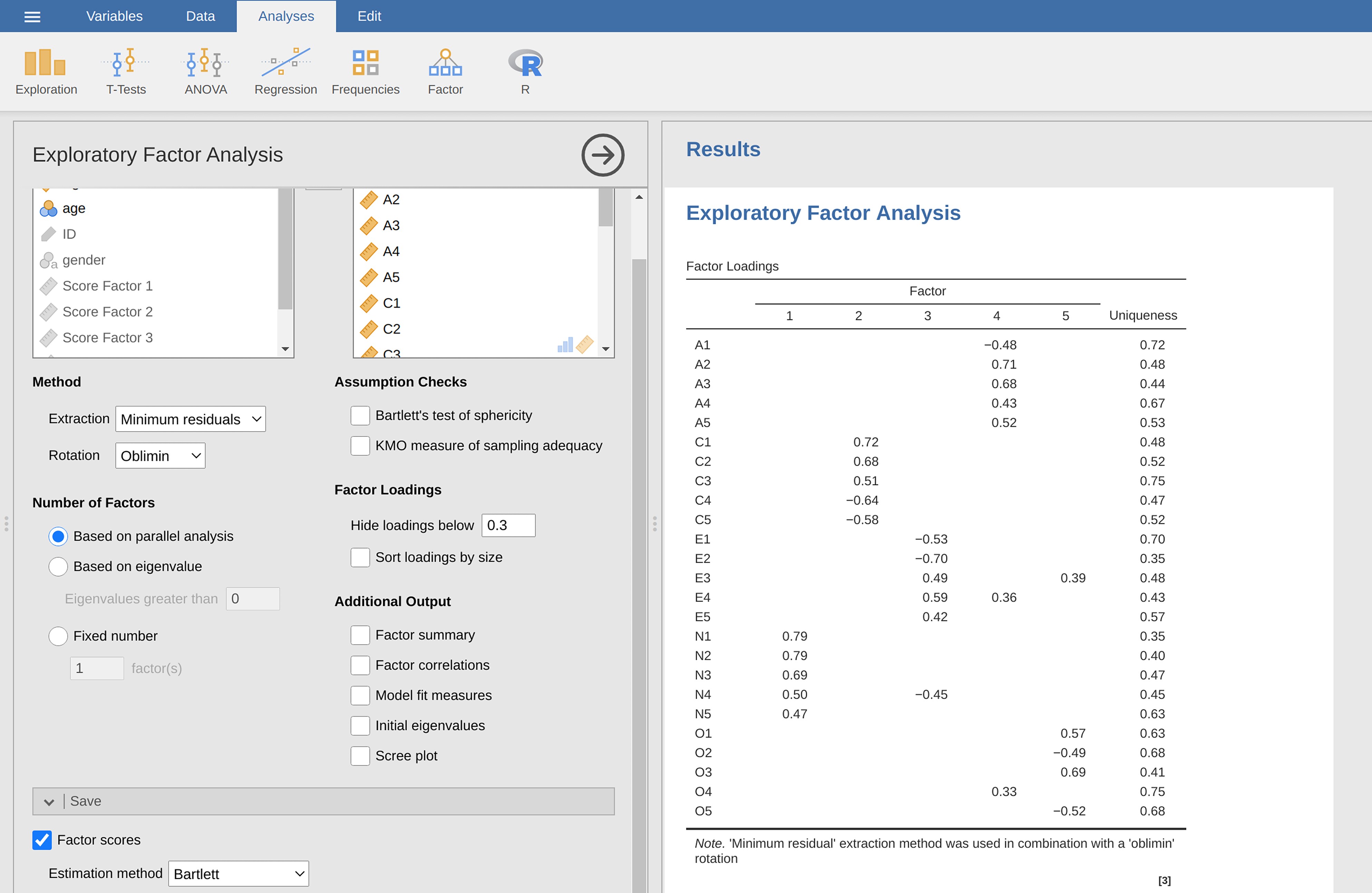
Abb. 204 Rj-Editor-Befehle für das Berechnen von optimal gewichteten Faktor-Scores für die Fünf-Faktoren-Lösung

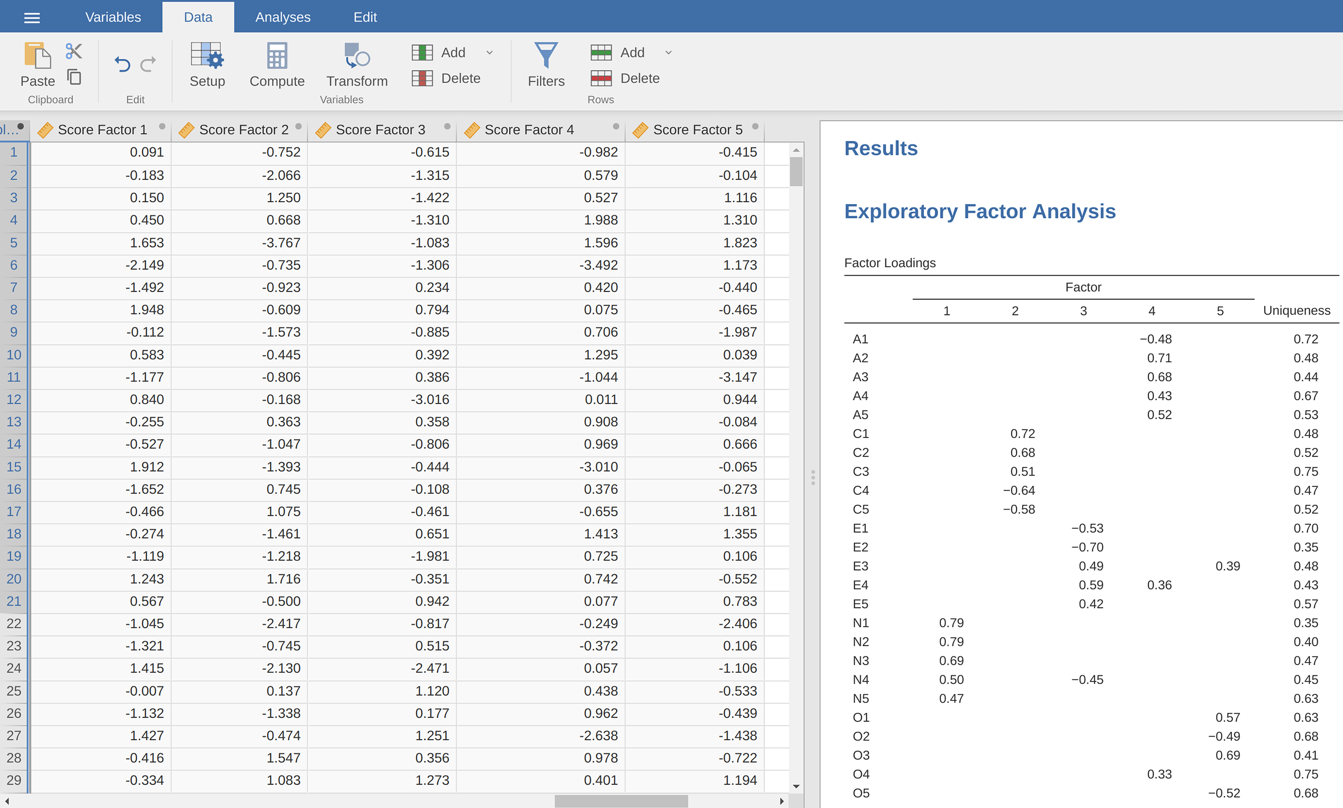
Abb. 205 Mit Hilfe der Befehle im Editor Rj erstellte Datendatei bfifactscores.csv, welche die fünf Faktor-Score-Variablen enthält. Beachten Sie, dass jede der neuen Faktor-Score-Variablen entsprechend der Reihenfolge der Faktoren in der Tabelle der Faktorladungen beschriftet ist.

Now you can go ahead and undertake further analyses, using either the factor- based scores (a mean scale score approach) or using the optimally-weighted factor scores calculated via the Rj editor. Your choice! For example, one thing you might like to do is see whether there are any gender differences in each of our personality scales. We did this for the Agreeableness score that we calculated using the factor-based score approach, and although the plot (see Abb. 206) showed that males were less agreeable than females, this was not a significant difference (Mann-Whitney U = 5760.5, p = 0.073).

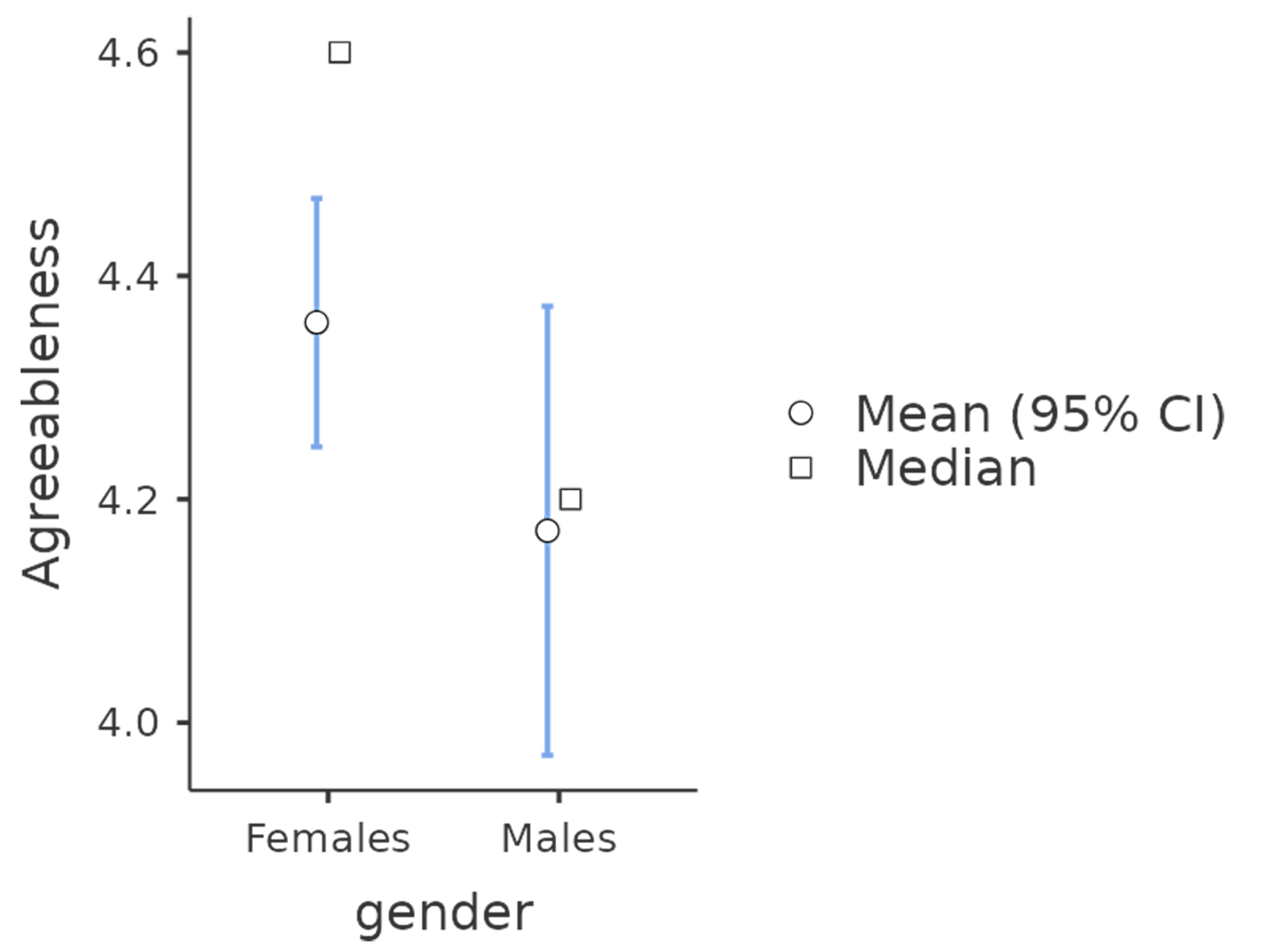
Abb. 206 Vergleich der Unterschiede zwischen Männern und Frauen in Bezug auf die Ausprägung auf dem Faktor „Verträglichkeit“

Berichten einer EFA

Hoffentlich konnten wir Ihnen einen Eindruck darüber vermitteln, was eine EFA ist und wie sie in jamovi durchgeführt wird. Wenn Sie Ihre EFA abgeschlossen haben, wie berichten Sie diese? Es gibt keine Standardmethode, um eine EFA zu berichten, und die Beispiele variieren je nach Disziplin und Forscher. Dennoch gibt es einige Informationen, die Sie in Ihren Bericht aufnehmen sollten:

1. Welches sind die theoretischen Grundlagen für den von Ihnen untersuchten Gegenstand und insbesondere was sind die Konstrukte, die Sie mittels der EFA untersuchen möchten?

2. A description of the sample (e.g., demographic information, sample size, sampling method).

3. Eine Beschreibung der Art der verwendeten Daten (z. B. nominal , kontinuierlich ) sowie Deskriptivstatistik für diese Variablen.

4. Beschreiben Sie, wie Sie beim Testen der Voraussetzungen für das Durchführen einer EFA vorgegangen sind. Dies sollte Details zu Sphärizitätsprüfungen (Bartlett) und Maßen der Stichprobenangemessenheit (KMO) umfassen.

5. Explain what FA extraction method (e.g., maximum likelihood) was used.

6. Erläutern Sie die Kriterien und den Prozess, nach denen entschieden wurde, wie viele Faktoren in der endgültigen Lösung extrahiert wurden und welche Items ausgewählt wurden. Erläutern Sie klar die Gründe für wichtige Entscheidungen während dieses Auswahlprozesses.

7. Erläutern Sie, welche Rotationsmethoden ausprobiert wurden, die Gründe dafür und die Ergebnisse.

8. Die endgültigen Faktorladungen sollten in den Ergebnissen in einer Tabelle angegeben werden. In dieser Tabelle sollte auch die Uniqueness (oder die Kommunalität) für jede Variable angegeben werden (in der letzten Spalte). Die Faktorladungen sollten mit beschreibenden Bezeichnungen zusätzlich zu den Item-Nummern angegeben werden. Die Korrelationen zwischen den Faktoren sollten ebenfalls angegeben werden, entweder am Ende dieser Tabelle oder in einer separaten Tabelle.

9. Es sollten aussagekräftige Namen für die extrahierten Faktoren angegeben werden. Es kann sein, dass Sie zuvor gewählte Faktornamen verwenden möchten. Es kann aber auch sein, dass Sie bei der Untersuchung der tatsächlichen Items und Faktoren denken, dass ein anderer Name besser geeignet ist.

---

[1]

Hilfreich ist, dass die Faktorladungen wie standardisierte Regressionskoeffizienten interpretiert werden können

[2]

A more advanced statistical technique, one which is beyond the scope of this book, undertakes regression modelling where latent factors are used in prediction models of other latent factors. This is called “structural equation modelling” and there are specific software programs and R packages dedicated to this approach.

[3]

An Eigen value indicates how much of the variance in the observed variables a factor accounts for. A factor with an Eigen value > 1 accounts for more variance than a single observed variable.

[4]

Oblique rotations provide two factor matrices, one called a structure matrix and one called a pattern matrix. In jamovi just the pattern matrix is shown in the results as this is typically the most useful for interpretation, though some experts suggest that both can be helpful. In a structure matrix coefficients show the relationship between the variable and the factors whilst ignoring the relationship of that factor with all the other factors (i.e., a zero-order correlation). Pattern matrix coefficients show the unique contribution of a factor to a variable whilst controlling for the effects of other factors on that variable (akin to standardized partial regression coefficient). Under orthogonal rotation, structure and pattern coefficients are the same.

[5]

In der Faktorenanalyse wird manchmal die „Kommunalität“ angegeben, d. h. der Anteil der Varianz in einer Variablen, der durch die Faktorenlösung erklärt wird. Die Uniqueness ist gleich (1 - Kommunalität).

[6]

Denken Sie daran, dass Sie gegebenenfalls zunächst einige Variablen invertieren müssen.