Forfatter av avsnitt: Danielle J. Navarro and David R. Foxcroft

Bekreftende faktoranalyse

So, our attempt to identify underlying latent factors using EFA with carefully selected questions from the personality item pool seemed to be pretty successful. The next step in our quest to develop a useful measure of personality is to check the latent factors we identified in the original EFA with a different sample. We want to see if the factors hold up, if we can confirm their existence with different data. This is a more rigorous check, as we will see. And it is called Confirmatory Factor Analysis (CFA) as we will, unsuprisingly, be seeking to confirm a pre-specificied latent factor structure.[1]

In CFA, instead of doing an analysis where we see how the data goes together in an exploratory sense, we instead impose a structure, like in Fig. 207, on the data and see how well the data fits our pre-specified structure. In this sense, we are undertaking a confirmatory analysis, to see how well a pre-specified model is confirmed by the observed data.

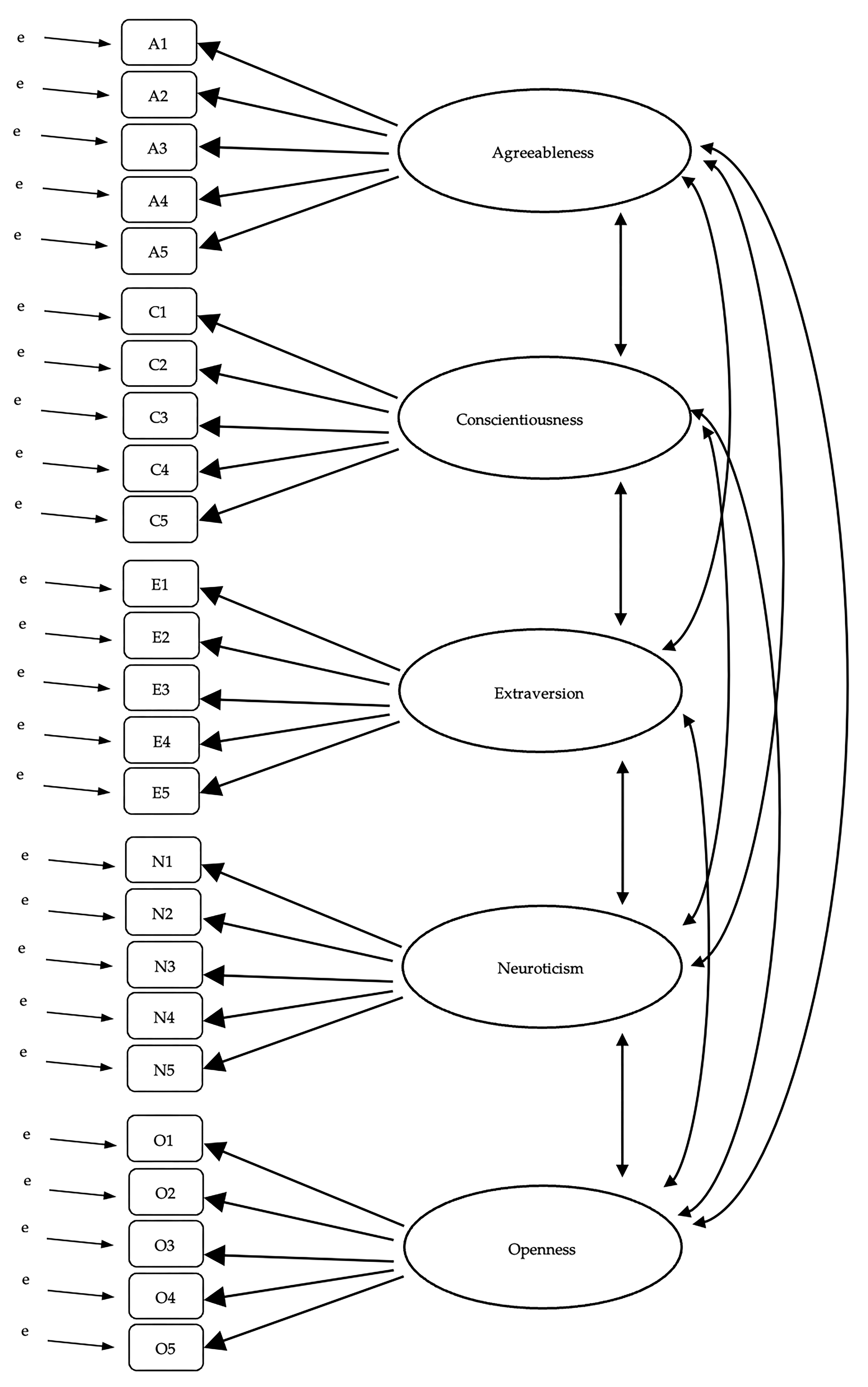
Fig. 207 Innledende forhåndsspesifisering av latent faktorstruktur for de fem personlighetsskalaene, til bruk i CFA

A straightforward confirmatory factor analysis (CFA) of the personality items would therefore specify five latent factors as shown in Fig. 207, each measured by five observed variables. Each variable is a measure of an underlying latent factor. For example, A1 is predicted by the underlying latent factor Agreeableness. And because A1 is not a perfect measure of the Agreeableness factor, there is an error term, e, associated with it. In other words, e represents the variance in A1 that is not accounted for by the Agreeableness factor. This is sometimes called measurement error.

The next step is to consider whether the latent factors should be allowed to correlate in our model. As mentioned earlier, in the psychological and behavioural sciences constructs are often related to each other, and we also think that some of our personality factors may be correlated with each other. So, in our model, we should allow these latent factors to covary, as shown by the double-headed arrows in Fig. 207.

At the same time, we should consider whether there is any good, systematic, reason for some of the error terms to be correlated with each other. One reason for this might be that there is a shared methodological feature for particular sub-sets of the observed variables such that the observed variables might be correlated for methodological rather than substantive latent factor reasons. We will return to this possibility in a later section but, for now, there are no clear reasons that we can see that would justify correlating some of the error terms with each other.

Without any correlated error terms, the model we are testing to see how well it fits with our observed data is just as specified in Fig. 207. Only parameters that are included in the model are expected to be found in the data, so in CFA all other possible parameters (coefficients) are set to zero. So, if these other parameters are not zero (for example there may be a substantial loading from A1 onto the latent factor Extraversion in the observed data, but not in our model) then we may find a poor fit between our model and the observed data.

CFA i jamovi

To set this CFA analysis up in jamovi, we open up the bfi_sample2 data set, check that the 25 variables are coded as ordinal (or continuous ; it will not make any difference for this analysis), and perform a CFA using the following steps:

• Select Factor → Confirmatory Factor Analysis from the Analyses tab to open the options panel where you can determine the settings for the CFA (Fig. 208).

• Select the five A variables and transfer them into the Factors box and give them the label “Agreeableness”.

• Create a new Factor in the Factors box and label it “Conscientiousness”. Select the five C variables and transfer them into the Factors box under the “Conscientiousness” label.

• Create another new Factor in the Factors box and label it “Extraversion”. Select the five E variables and transfer them into the Factors box under the “Extraversion” label.

• Create another new Factor in the Factors box and label it “Neuroticism”. Select the five N variables and transfer them into the Factors box under the “Neuroticism” label.

• Create another new Factor in the Factors box and label it “Openness”. Select the five O variables and transfer them into the Factors box under the “Openness” label.

• Check other appropriate options, the defaults are OK for this initial work through, though you might want to check the Path diagram option under Plots to see jamovi produce a (fairly) similar diagram to our Fig. 207.

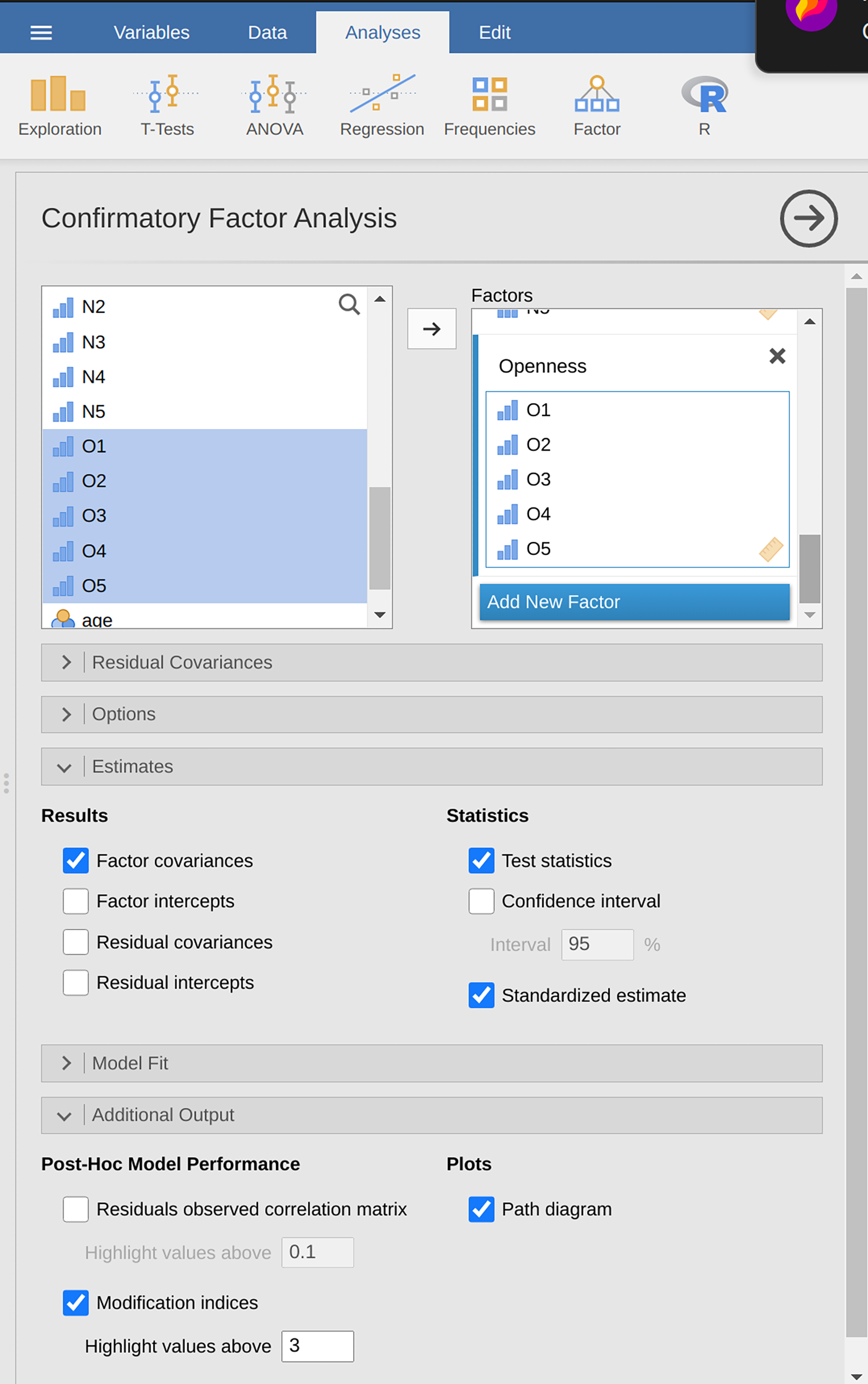
Fig. 208 Analysepanel med innstillinger for gjennomføring av en konfirmatorisk faktoranalyse (CFA) i jamovi

Once we have set up the analysis we can turn our attention to the jamovi results panel and see what is what. The first thing to look at is model fit (Fig. 209) as this tells us how good a fit our model is to the observed data. NB in our model only the pre-specified covariances are estimated, including the factor correlations by default. Everything else is set to zero.

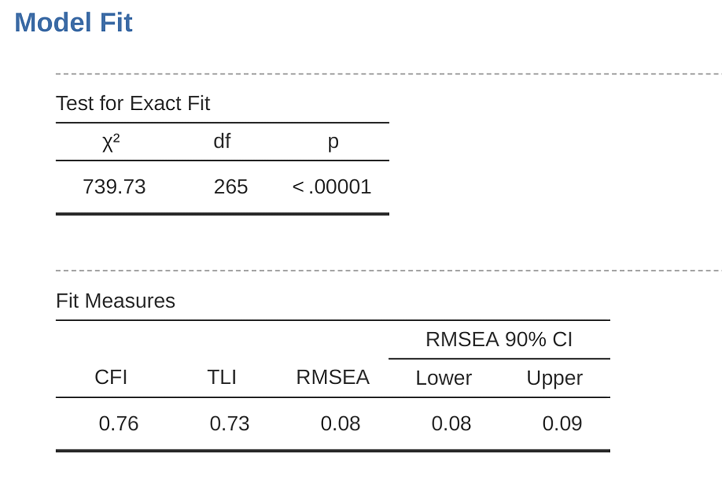
Fig. 209 Tabell med Model Fit-resultater for den spesifiserte CFA-modellen i jamovi

Det finnes flere måter å vurdere modelltilpasning på. Den første er en χ²-statistikk som, hvis den er liten, indikerer at modellen passer godt til dataene. χ²-statistikken som brukes til å vurdere modelltilpasning, er imidlertid ganske følsom for utvalgsstørrelsen, noe som betyr at med et stort utvalg gir en god nok tilpasning mellom modellen og dataene nesten alltid en stor og signifikant (p < 0,05) χ²-verdi.

Derfor trenger vi andre måter å vurdere modelltilpasning på. jamovi tilbyr flere slike metoder som standard. Disse er Comparative Fit Index (CFI), Tucker Lewis Index (TLI) og Root Mean Square Error of Approximation (RMSEA) sammen med 90%-konfidensintervall for RMSEA. Noen nyttige tommelfingerregler er at en tilfredsstillende tilpasning indikeres av CFI > 0,9, TLI > 0,9 og RMSEA på rundt 0,05 til 0,08. En god tilpasning er CFI > 0,95, TLI > 0,95 og RMSEA og øvre KI for RMSEA < 0,05.

So, looking at Fig. 209, we can see that the χ²-value is large and highly significant. Our sample size is not too large, so this possibly indicates a poor fit. The CFI is 0.762 and the TLI is 0.731, indicating poor fit between the model and the data. The RMSEA is 0.085 with a 90% confidence interval from 0.077 to 0.092, again this does not indicate a good fit.

Ganske skuffende, hva? Men kanskje ikke så overraskende med tanke på at i den tidligere EFA-en, da vi kjørte med et lignende datasett (avsnitt Eksplorerende faktoranalyse), ble bare rundt halvparten av variansen i dataene forklart av femfaktormodellen.

Let us go on to look at the factor loadings and the factor covariance estimates, shown in Fig. 210 and Fig. 211. The Z-statistic and p-value for each of these parameters indicates they make a reasonable contribution to the model (i.e., they are not zero) so there does not appear to be any reason to remove any of the specified variable-factor paths, or factor-factor correlations from the model. Often the standardized estimates are easier to interpret, and these can be specified under the Estimates option. These tables can usefully be incorporated into a written report or scientific article.

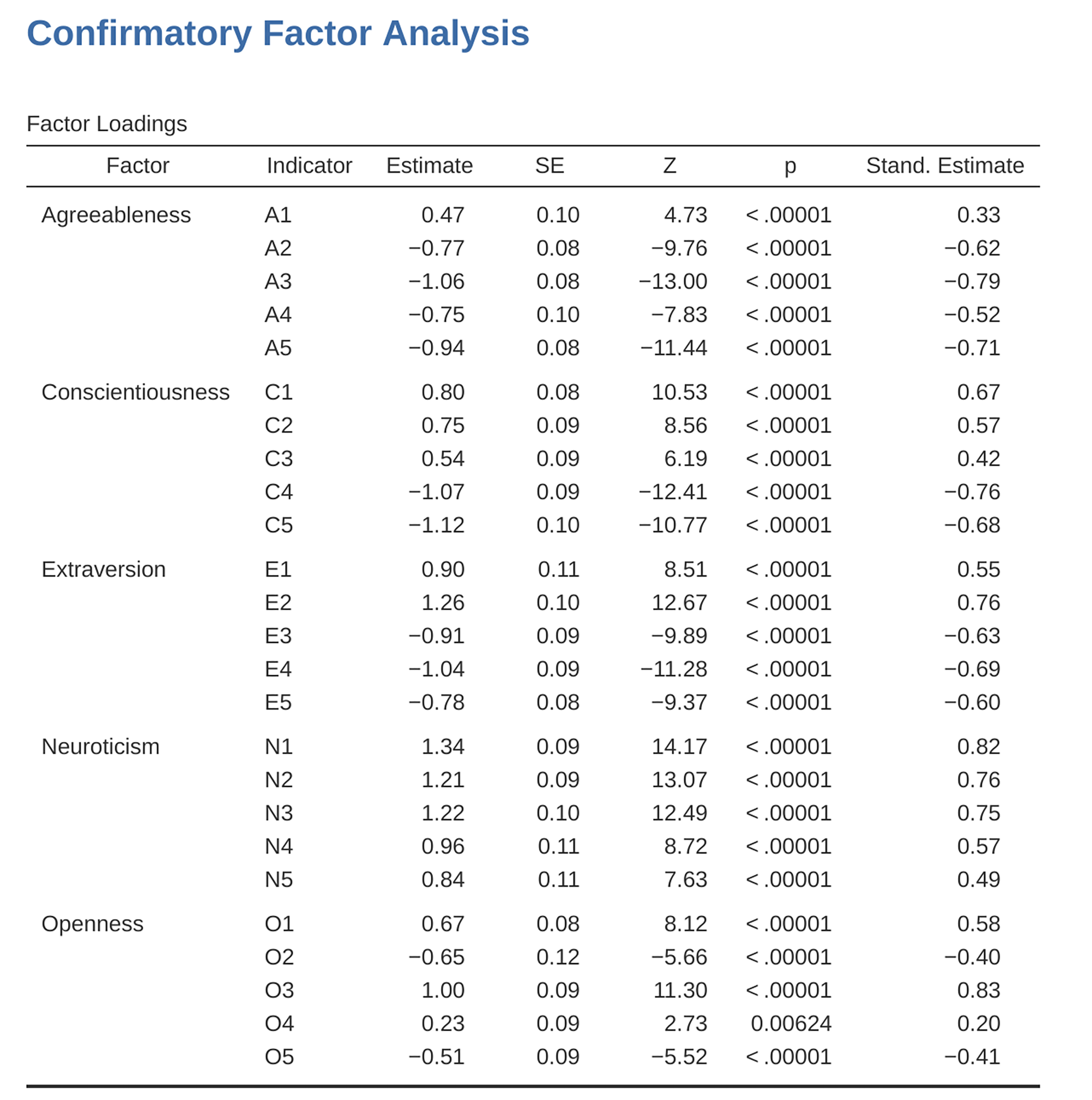
Fig. 210 Tabell med Factor Loadings for den spesifiserte CFA-modellen i jamovi

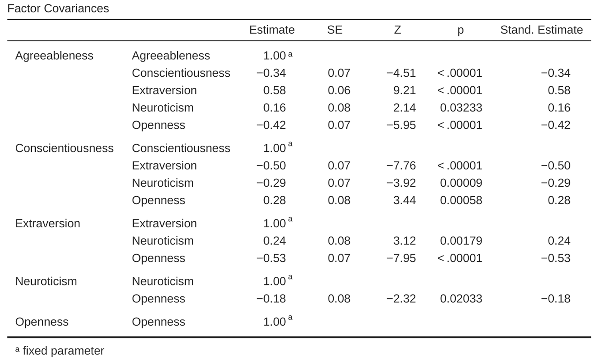
Fig. 211 Tabell med Factor Covariances for den spesifiserte CFA-modellen i jamovi

How could we improve the model? One option is to go back a few stages and think again about the items / measures we are using and how they might be improved or changed. Another option is to make some post-hoc tweaks to the model to improve the fit. One way of doing this is to use Modification indices, specified as an Additional Output option in jamovi (see Fig. 212).

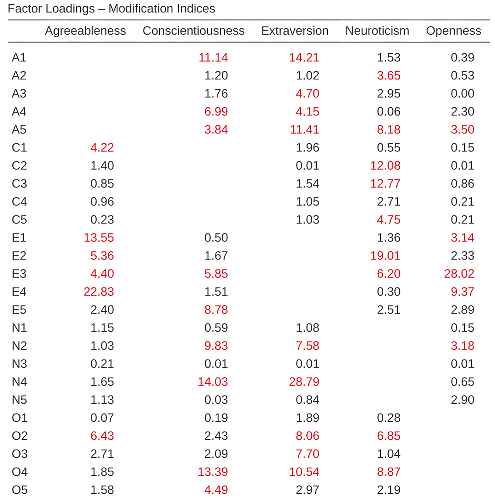
Fig. 212 Tabell med Factor Loadings Modification Indices for den spesifiserte CFA-modellen i jamovi

What we are looking for is the highest modification index (MI) value. We would then judge whether it makes sense to add that additional term into the model, using a post-hoc rationalisation. For example, we can see in Fig. 212 that the largest MI for the factor loadings that are not already in the model is a value of 28.786 for the loading of N4 (“Often feel blue”) onto the latent factor Extraversion. This indicates that if we add this path into the model then the χ²-value will reduce by around the same amount.

But in our model adding this path arguably does not really make any theoretical or methodological sense, so it is not a good idea (unless you can come up with a persuasive argument that “Often feel blue” measures both Neuroticism and Extraversion). I can not think of a good reason. But, for the sake of argument, let us pretend it does make some sense and add this path into the model. Go back to the CFA analysis window (see Fig. 208) and add N4 into the Extraversion factor. The results of the CFA will now change (not shown); the χ²-value has come down to around 709 (a drop of around 30, roughly similar to the size of the MI) and the other fit indices have also improved, though only a bit. But it is not enough: it is still not a good fitting model.

Hvis du legger til nye parametere i en modell ved hjelp av MI-verdiene, må du alltid sjekke MI-tabellene på nytt etter hvert nye tillegg, ettersom MI-verdiene oppdateres hver gang.

There is also a Table of Residual Covariances Modification Indices produced by jamovi (Fig. 213). In other words, a table showing which correlated errors, if added to the model, would improve the model fit the most. It is a good idea to look across both MI tables at the same time, spot the largest MI, think about whether the addition of the suggested parameter can be reasonably justified and, if it can, add it to the model. And then you can start again looking for the biggest MI in the re-calculated results.

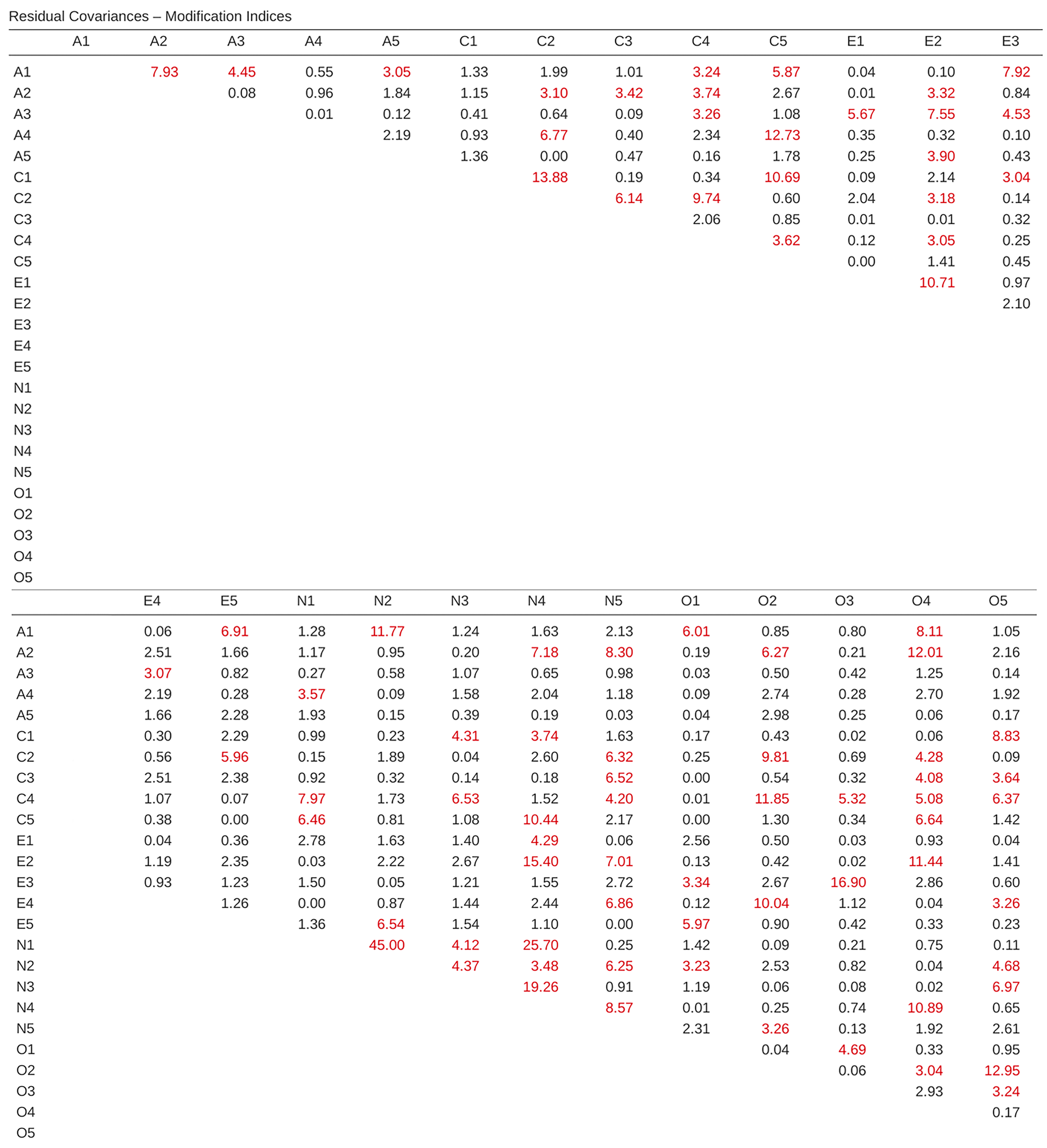
Fig. 213 Tabell med Residual Covariances Modification Indices for den spesifiserte CFA-modellen i jamovi

You can keep going this way for as long as you like, adding parameters to the model based on the largest MI, and eventually you will achieve a satisfactory fit. But there will also be a strong possibility that in doing this you will have created a monster! A model that is ugly and deformed and does not have any theoretical sense or purity. In other words, be very careful!

So far, we have checked out the factor structure obtained in the EFA using a second sample and CFA. Unfortunately, we did not find that the factor structure from the EFA was confirmed in the CFA, so it is back to the drawing board as far as the development of this personality scale goes.

Selv om det noen ganger kan være gode grunner til å la residuene samvariere (eller korrelere), var det ingen slike grunner til å «optimalisere» CFA-en for modellen som vi definerte ved å inkludere ytterligere faktorladninger eller residualkovarianser ved hjelp av modifikasjonsindekser. La oss likevel diskutere hvordan vi kan rapportere resultatene av en CFA (med en mer tilpasset modell).

Rapportering av en CFA

Det finnes ingen formell standardmåte å skrive en CFA på, og eksemplene har en tendens til å variere fra fagfelt til fagfelt og forsker til forsker. Når det er sagt, finnes det likevel noen standardopplysninger som bør inkluderes i rapporten:

1. En teoretisk og empirisk begrunnelse for den hypotetiske modellen.

2. A complete description of how the model was specified (e.g., the indicator variables for each latent factor, covariances between latent variables, and any correlations between error terms). A path diagram, like the one in Fig. 207 would be good to include.

3. A description of the sample (e.g., demographic information, sample size, sampling method).

4. En beskrivelse av hvilken type data som er brukt (f.eks. nominell , kontinuerlig ) og deskriptivstatistikk.

5. Tester av forutsetninger og estimeringsmetode.

6. En beskrivelse av manglende data og hvordan de manglende dataene ble håndtert.

7. Programvaren og versjonen som ble brukt til å tilpasse modellen.

8. Mål og kriterier som brukes for å bedømme modelltilpasning.

9. Eventuelle endringer i den opprinnelige modellen basert på modelltilpasning eller modifikasjonsindekser.

10. Alle parameterestimater (dvs. ladninger, feilvarianser, latente (ko)varianser) og deres standardfeil, sannsynligvis i en tabell.

---

[1]

Som en parentes bemerket kunne vi, gitt at vi hadde en ganske sikker idé ut fra de første «antatte» faktorene våre, bare ha gått rett til CFA og hoppet over EFA-trinnet. Hvorvidt man bruker EFA og deretter går videre til CFA, eller om man går rett til CFA, er et spørsmål om skjønn og hvor sikker man er på at modellen er riktig i utgangspunktet (med hensyn til antall faktorer og variabler). På et tidlig stadium i utviklingen av skalaer eller identifiseringen av underliggende latente konstrukter har forskere en tendens til å bruke EFA. Senere, når de nærmer seg en endelig skala, eller hvis de ønsker å sjekke en etablert skala i et nytt utvalg, er CFA et godt alternativ.