Forfatter av avsnitt: Danielle J. Navarro and David R. Foxcroft

Eksplorerende faktoranalyse

Eksplorerende faktoranalyse (EFA) er en statistisk teknikk for å avdekke eventuelle skjulte latente faktorer som kan utledes fra våre observerte data. Denne teknikken beregner i hvilken grad et sett med målte variabler, for eksempel V1, V2, V3, V4 og V5, kan representeres som mål på en underliggende latent faktor. Denne latente faktoren kan ikke måles gjennom bare én observert variabel, men kommer i stedet til uttrykk i de sammenhengene den forårsaker i et sett med observerte variabler.

In Fig. 196 each observed variable V is “caused” to some extent by the underlying latent factor (F), depicted by the coefficients b1 to b5 (also called factor loadings). Each observed variable also has an associated error term, e1 to e5. Each error term is the variance in the associated observed variable, V_i, that is unexplained by the underlying latent factor.

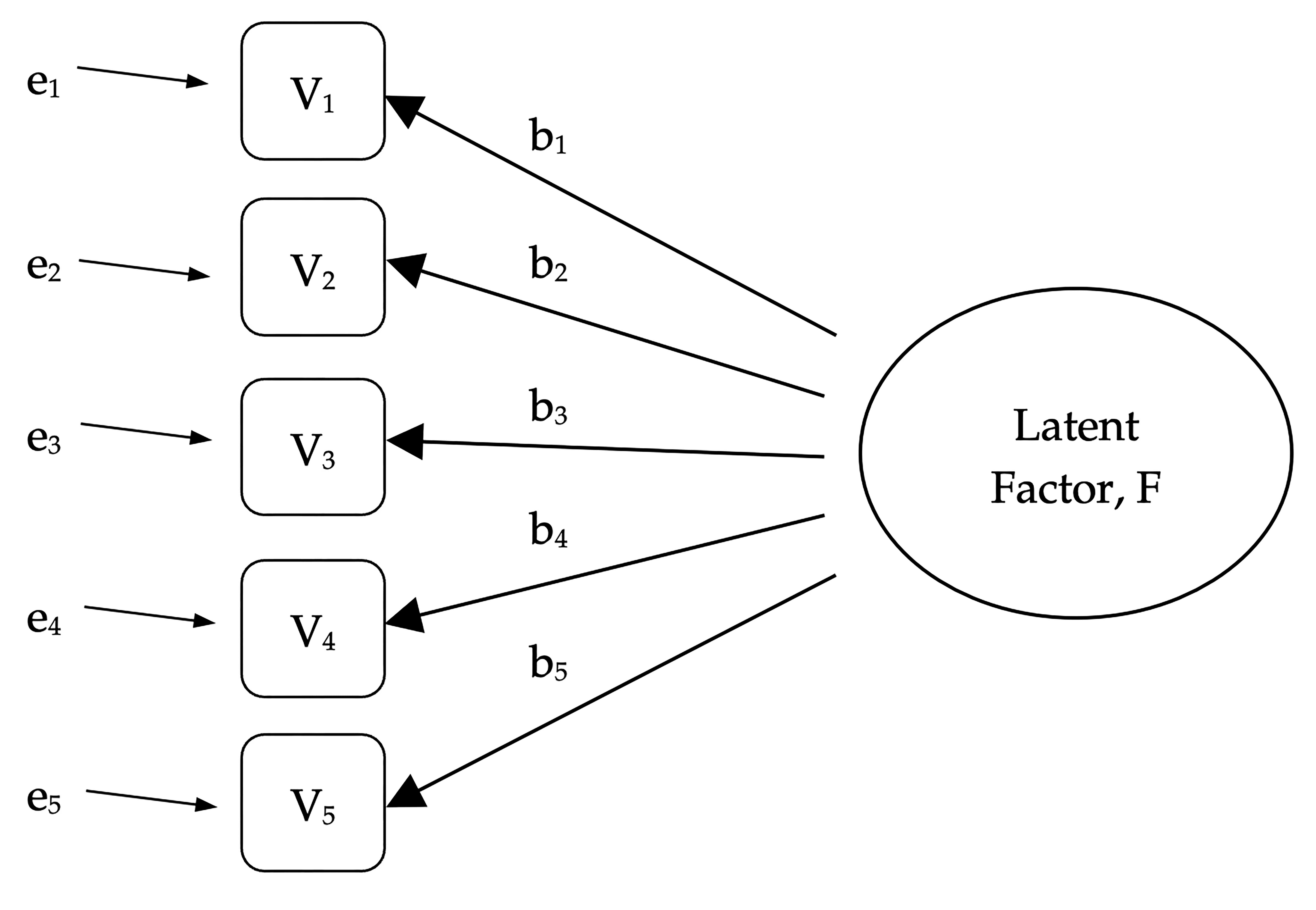
Fig. 196 Latent faktor som ligger til grunn for forholdet mellom flere observerte variabler

In Psychology, latent factors represent psychological phenomena or constructs that are difficult to directly observe or measure. For example, personality, or intelligence, or thinking style. In the example in Fig. 196, we may have asked people five specific questions about their behaviour or attitudes, and from that we are able to get a picture about a personality construct called, for example, extraversion. A different set of specific questions may give us a picture about an individual’s introversion, or their conscientiousness.

Here is another example: we may not be able to directly measure statistics anxiety, but we can measure whether statistics anxiety is high or low with a set of questions in a questionnaire. For example, “Q1: Doing the assignment for a statistics course”, “Q2: Trying to understand the statistics described in a journal article”, and “Q3: Asking the lecturer for help in understanding something from the course”, etc., each rated from low anxiety to high anxiety. People with high statistics anxiety will tend to give similarly high responses on these observed variables because of their high statistics anxiety. Likewise, people with low statistics anxiety will give similar low responses to these variables because of their low statistics anxiety.

In Exploratory Factor Analysis (EFA), we are essentially exploring the correlations between observed variables to uncover any interesting, important underlying (latent) factors that are identified when observed variables covary. We can use statistical software to estimate any latent factors and to identify which of our variables have a high loading[1] (e.g., loading > 0.5) on each factor, suggesting they are a useful measure, or indicator, of the latent factor. Part of this process includes a step called rotation, which to be honest is a pretty weird idea but luckily we do not have to worry about understanding it; we just need to know that it is helpful because it makes the pattern of loadings on different factors much clearer. As such, rotation helps with seeing more clearly which variables are linked substantively to each factor. We also need to decide how many factors are reasonable given our data, and helpful in this regard is something called Eigen values. We will come back to this in a moment, after we have covered some of the main assumptions of EFA.

Sjekk av forutsetninger

There are a couple of assumptions that need to be checked as part of the analysis. The first assumption is sphericity, which essentially checks that the variables in your data set are correlated with each other to the extent that they can potentially be summarised with a smaller set of factors. Bartlett’s test for sphericity checks whether the observed correlation matrix diverges significantly from a zero (or null) correlation matrix. So, if Bartlett’s test is significant (p < 0.05), this indicates that the observed correlation matrix is significantly divergent from the null, and is therefore suitable for EFA.

Den andre forutsetningen er trekkelighet av utvalg (sampling adequacy) og kontrolleres ved hjelp av Kaiser-Meyer-Olkin (KMO) Measure of Sampling Adequacy (MSA). KMO-indeksen er et mål på hvor stor andel av variansen blant de observerte variablene som kan være felles varians. Ved hjelp av partielle korrelasjoner sjekker den om det finnes faktorer som bare lader på to spørsmål. Vi ønsker sjelden, om noen gang, at EFA skal produsere mange faktorer som bare lader på to spørsmål hver. KMO handler om tilstrekkelighet av utvalg, fordi partielle korrelasjoner vanligvis oppstår når utvalget ikke er tilstrekkelig. Hvis KMO-indeksen er høy (≈ 1), er EFA effektiv, mens hvis KMO er lav (≈ 0), er EFA ikke relevant. KMO-verdier under 0,5 indikerer at EFA ikke er egnet, og en KMO-verdi på 0,6 bør være til stede før EFA anses som egnet. Verdier mellom 0,5 og 0,7 anses som adekvate, verdier mellom 0,7 og 0,9 er gode, og verdier mellom 0,9 og 1,0 er utmerkede.

Hva er EFA bra for?

If the EFA has provided a good solution (i.e., a good factor model), then we need to decide what to do with our shiny new factors. Researchers often use EFA during psychometric scale development. They will develop a pool of questionnaire items that they think relate to one or more psychological constructs, use EFA to see which items “go together” as latent factors, and then they will assess whether some items should be removed because they do not usefully or distinctly measure one of the latent factors.[2]

I tråd med denne tilnærmingen er en annen konsekvens av EFA å kombinere variablene som lader på forskjellige faktorer, til en faktorskår, også kjent som en skalaskår. Det finnes to alternativer for å kombinere variabler til en skalapoengsum:

• Opprett en ny variabel med en poengsum vektet med faktorladningene for hvert spørsmål som bidrar til faktoren.

• Opprett en ny variabel basert på hvert spørsmål som bidrar til faktoren, men vekt dem likt.

In the first option each item’s contribution to the combined score depends on how strongly it relates to the factor. In the second option we typically just average across all the items that contribute substantively to a factor to create the combined scale score variable. Which to choose is a matter of preference, though a disadvantage with the first option is that loadings can vary quite a bit from sample to sample, and in behavioural and health sciences we are often interested in developing and using composite questionnaire scale scores across different studies and different samples. In which case it is reasonable to use a composite measure that is based on the substantive items contributing equally rather than weighting by sample specific loadings from a different sample. In any case, understanding a combined variable measure as an average of items is simpler and more intuitive than using a sample specific optimally-weighted combination. But let us not get ahead of ourselves; what we should really focus on now is how to do an EFA in jamovi.

EFA i jamovi

First, we need some data. Twenty-five personality self-report items (see Table 18) taken from the International Personality Item Pool (https://ipip.ori.org) were included as part of the Synthetic Aperture Personality Assessment web-based personality assessment (SAPA; https://sapa-project.org) project. The 25 items are short phrases that one should respond to by indicating how accurately the statement describes one’s typical behaviour or attitudes. The items are organized by five putative factors: Agreeableness, Conscientiousness, Extraversion, Neuroticism, and Openness.

Table 18 Tjuefem observerte variabeler / spørsmål organisert etter fem antatte personlighetsfaktorer i datasettet bfi_sample. Hvis det er en R i den andre kolonnen, er spørsmålet reversert.

Navn		Spørsmål
A1	R	Er likegyldig til andres følelser.
A2		Spør om andres velvære.
A3		Vet hvordan du kan trøste andre.
A4		Elsker barn.
A5		Få folk til å føle seg trygge.
C1		Jeg er krevende i arbeidet mitt.
C2		Fortsett til alt er perfekt.
C3		Gjør ting i henhold til en plan.
C4	R	Gjør ting på en halvveis måte.
C5	R	Jeg kaster bort tiden min.
E1	R	Ikke snakk så mye.
E2	R	Synes det er vanskelig å ta kontakt med andre.
E3		Vet hvordan du skal fange folk.
E4		Det er lett å få venner.
E5		Ta ansvar.
N1		Har lett for å bli sint.
N2		Blir lett irritert.
N3		Har hyppige humørsvingninger.
N4		Føler meg ofte nedfor.
N5		Får lett panikk.
O1		Jeg er full av ideer.
O2	R	Unngå vanskelig lesestoff.
O3		Løft samtalen opp på et høyere nivå.
O4		Bruk tid på å reflektere over ting.
O5	R	Vil ikke gå dypt inn i et emne.

Dataene ble samlet inn ved hjelp av en 6-punkts svarskala:

1. Svært unøyaktig

2. Moderat unøyaktig

3. Litt unøyaktig

4. Litt nøyaktig

5. Moderat nøyaktig

6. Veldig nøyaktig.

Et utvalg på N = 250 svar finnes i datasettet bfi_sample. I tillegg til svarene inneholder datasettet tre andre kolonner: ID (respondentens ID, et femsifret nummer) samt respondentens alder (age) og kjønn (gender).

As researchers, we are interested in exploring the data to see whether there are some underlying latent factors that are measured reasonably well by the 25 observed variables in the bfi_sample data set. Open it up and check that the 25 variables are coded as continuous variables (technically they are ordinal though for EFA in jamovi it mostly does not matter, except if you decide to calculate weighted factor scores in which case continuous variables are needed). To perform an EFA in jamovi:

• Select Factor → Exploratory Factor Analysis from the Analyses tab to open the options panel where you can determine the settings for the EFA (Fig. 197).

• Velg de 25 personlighetsspørsmålene, og overfør dem til boksen Variables.

• Check appropriate options, including Assumption Checks, but also Rotation under Method, Number of Factors to extract, and Additional Output options (see Fig. 197 for suggested options for this illustrative EFA, and please note that the Rotation under Method and Number of Factors extracted is typically adjusted by the researcher during the analysis to find the best result, as described below).

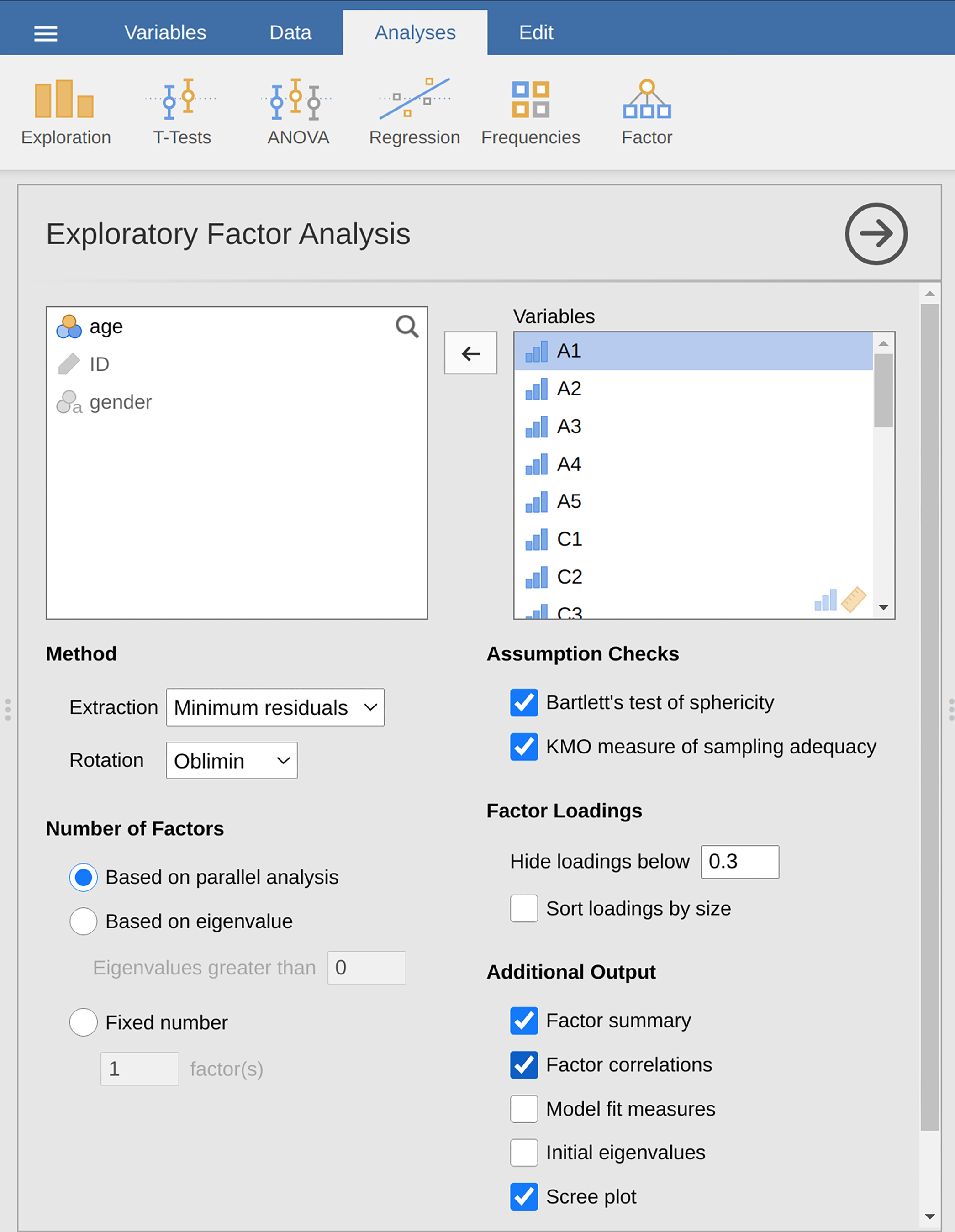
Fig. 197 Analysepanel med innstillingene for å gjennomføre en eksplorerende faktoranalyse (EFA) i jamovi

First, check the assumptions (Fig. 198). You can see that (1) Bartlett’s test of sphericity is significant, so this assumption is satisfied; and (2) the KMO measure of sampling adequacy (MSA) is 0.81 overall, suggesting good sampling adequacy. No problems here then!

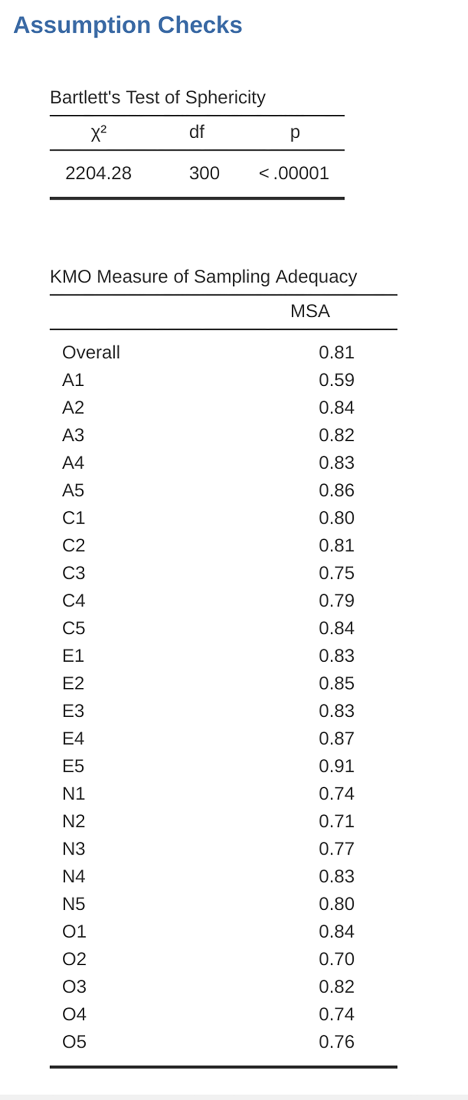
Fig. 198 jamovi EFA-forutsetningssjekker for personlighetsspørreskjemaet

Det neste du må sjekke, er hvor mange faktorer du skal bruke (eller «ekstrahere» fra dataene). Tre ulike tilnærminger er tilgjengelige:

• En konvensjon er å velge alle komponenter med Eigen-verdier større enn 1.[3] Dette vil gi oss fire faktorer med våre data (prøv det og se).

• Examination of the scree plot, as in Fig. 199, lets you identify the “point of inflection”. This is the point at which the slope of the scree curve clearly levels off, below the “elbow”. This would give us five factors with our data. Interpreting scree plots is a bit of an art: in Fig. 199 there is a noticeable step from five to seix factors, but in other scree plots you look at it will not be so clear cut.

• Ved hjelp av en parallell analyseteknikk sammenlignes de oppnådde Eigen-verdiene med de som ville blitt oppnådd fra tilfeldige data. Antallet faktorer som trekkes ut, er antallet med Eigen-verdier som er større enn det som ville blitt funnet med tilfeldige data.

Fig. 199 Scree plot av personlighetsdataene i EFA i jamovi, som viser en merkbar bøyning og utflating etter punkt 5 («albuen»)

Den tredje tilnærmingen er god ifølge Fabrigar et al. (1999), selv om forskere i praksis har en tendens til å se på alle tre og deretter gjøre en vurdering av hvor mange faktorer som er lettest eller mest nyttig å tolke. Dette kan forstås som «meningsfullhetskriteriet», og forskere vil typisk, i tillegg til løsningen fra en av tilnærmingene ovenfor, undersøke løsninger med en eller to faktorer til eller færre. Deretter velger de den løsningen som gir mest mening for dem.

At the same time, we should also consider the best way to rotate the final solution. There are two main approaches to rotation: orthogonal (e.g., Varimax) rotation forces the selected factors to be uncorrelated, whereas oblique (e.g., Oblimin) rotation allows the selected factors to be correlated. Dimensions of interest to psychologists and behavioural scientists are not often dimensions we would expect to be orthogonal, so oblique solutions are arguably more sensible.[4]

Practically, if in an oblique rotation the factors are found to be substantially correlated (positive or negative, and > 0.3), as in Fig. 200 where a correlation between two of the extracted factors is 0.31, then this would confirm our intuition to prefer oblique rotation. If the factors are, in fact, correlated, then an oblique rotation will produce a better estimate of the true factors and a better simple structure than will an orthogonal rotation. And, if the oblique rotation indicates that the factors have close to zero correlations between one another, then the researcher can go ahead and conduct an orthogonal rotation (which should then give about the same solution as the oblique rotation).

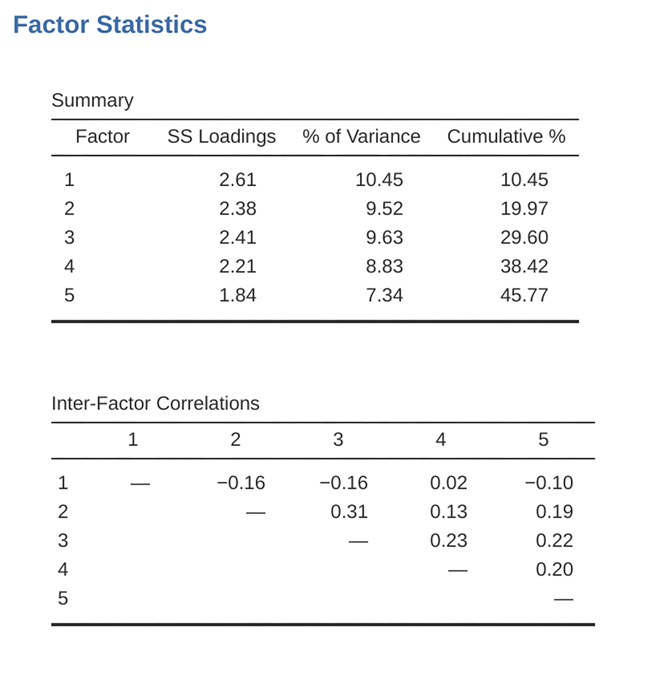
Fig. 200 Faktorsammendragsstatistikk og korrelasjoner for en femfaktorløsning i EFA utført i jamovi

On checking the correlation between the extracted factors at least one correlation was greater than 0.3 (Fig. 200), so an oblique (Oblimin) rotation of the five extracted factors is preferred. We can also see in Fig. 200 that the proportion of overall variance in the data that is accounted for by the five factors is 46%. Factor 1 accounts for around 10% of the variance, factors 2 to 4 around 9% each, and factor 5 just over 7%. This is not great; it would have been better if the overall solution accounted for a more substantive proportion of the variance in our data.

Vær oppmerksom på at du i hver EFA potensielt kan ha like mange faktorer som observerte variabler, men at hver ekstra faktor du inkluderer, vil tilføre en mindre mengde forklart varians. Hvis de første faktorene forklarer en god del av variansen i de opprinnelige 25 variablene, er disse faktorene helt klart en nyttig, enklere erstatning for de 25 variablene. Du kan droppe resten uten å miste for mye av den opprinnelige variabiliteten. Men hvis det for eksempel kreves 18 faktorer for å forklare mesteparten av variansen i de 25 variablene, kan du like gjerne bare bruke de opprinnelige 25.

Fig. 201 shows the factor loadings. That is, how the 25 different personality items load onto each of the five selected factors. We have hidden loadings less than 0.3 (set in the options shown in Fig. 197).

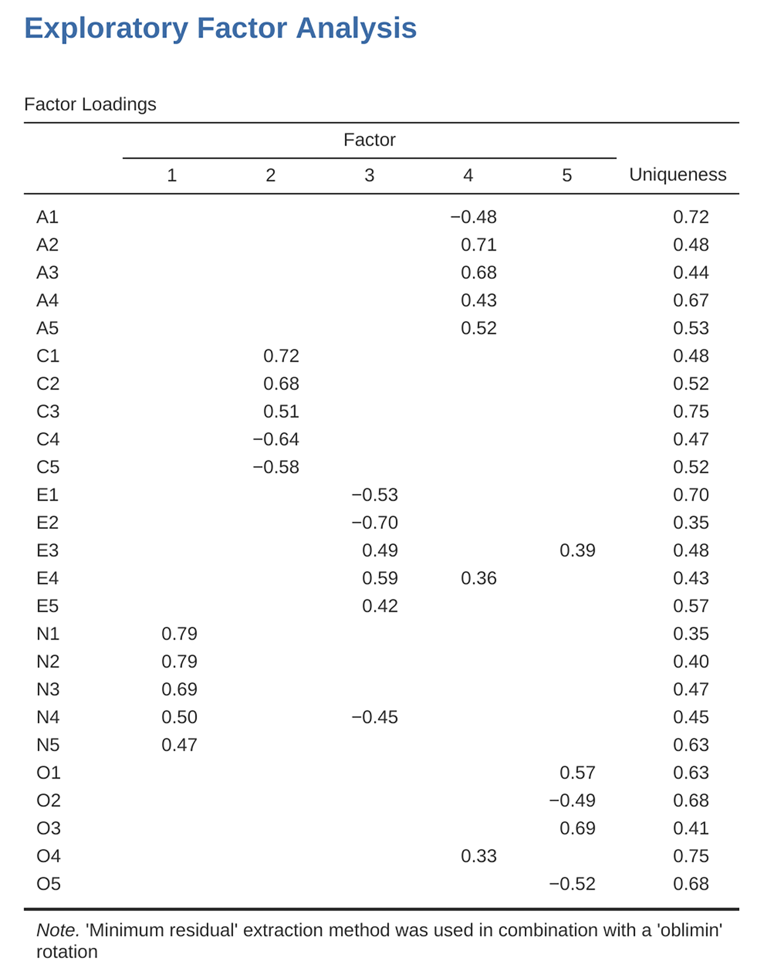
Fig. 201 Faktorladninger for en femfaktorløsning i EFA utført i jamovi

For factors 1, 2, 3 and 4 the pattern of factor loadings closely matches the putative factors specified in Table 18. Phew! And factor 5 is pretty close, with four of the five observed variables that putatively measure “Openness” loading pretty well onto the factor. Variable O4 does not quite seem to fit though, as the factor solution in Fig. 201 suggests that it loads onto factor 4 (albeit with a relatively low loading) but not substantively onto factor 5.

The other thing to note is that those variables that were denoted as “R: reverse coding” in Table 18 are those that have negative factor loadings. Take a look at the items A1 (“Am indifferent to the feelings of others”) and A2 (“Inquire about others’ well-being”). We can see that a high score on A1 indicates low Agreeableness, whereas a high score on A2 (and all the other A-variables for that matter) indicates high Agreeableness. Therefore A1 will be negatively correlated with the other A-variables, and this is why it has a negative factor loading, as shown in Fig. 201.

We can also see in Fig. 201 the Uniqueness of each variable. Uniqueness is the proportion of variance that is “unique” to the variable and not explained by the factors.[5] For example, 72% of the variance in A1 is not explained by the factors in the five factor solution. In contrast, N1 has relatively low variance not accounted for by the factor solution (35%). Note that the greater the Uniqueness, the lower the relevance or contribution of the variable in the factor model.

To be honest, it is unusual to get such a neat solution in EFA. It is typically quite a bit more messy than this, and often interpreting the meaning of the factors is more challenging. It is not often that you have such a clearly delineated item pool. More often you will have a whole heap of observed variables that you think may be indicators of a few underlying latent factors, but you do not have such a strong sense of which variables are going to go where!

So, we seem to have a pretty good five factor solution, albeit accounting for a relatively low overall proportion of the observed variance. Let us assume we are happy with this solution and want to use our factors in further analysis. The straightforward option is to calculate an overall (average) score for each factor by adding together the score for each variable that loads substantively onto the factor and then dividing by the number of variables. For each person in our data set that would mean, for example for the Agreeableness factor, adding together A1 + A2 + A3 + A4 + A5, and then dividing by 5.[6] In essence, this means that the factor score we have calculated is based on equally weighted scores from each of the included variables. We can do this in jamovi in two steps:

1. Recode A1 into A1R by reverse scoring the values in the variable (i.e., 6 = 1; 5 = 2; 4 = 3; 3 = 4; 2 = 5; 1 = 6) using the jamovi transform variable function (see Fig. 202).

2. Compute a new variable, called Agreeableness, by calculating the mean of A1R, A2, A3, A4 and A5. Do this using the jamovi Compute command to create a new variable (see Fig. 203).

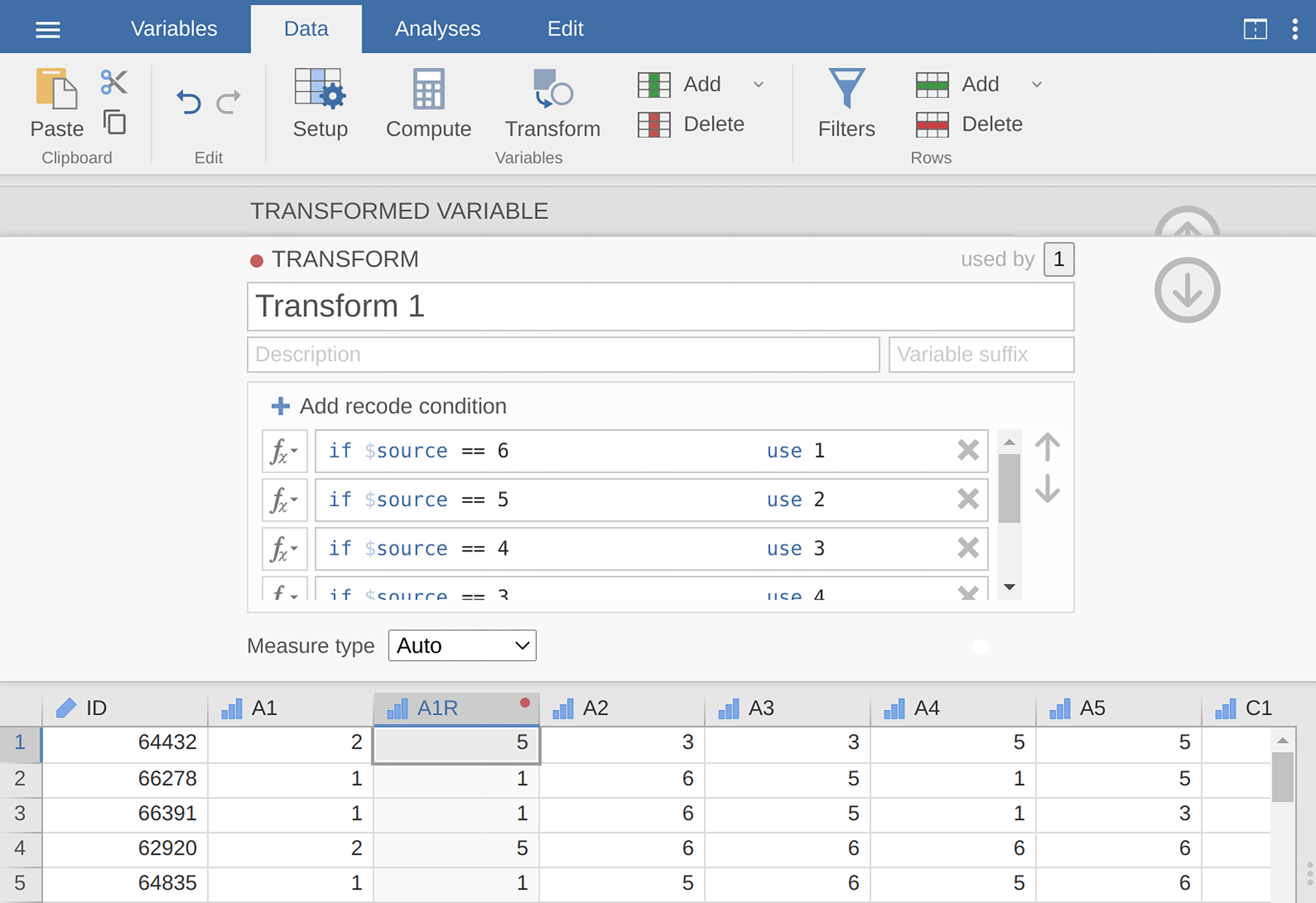
Fig. 202 Omkoding av variabel ved hjelp av Transform-kommandoen i jamovi

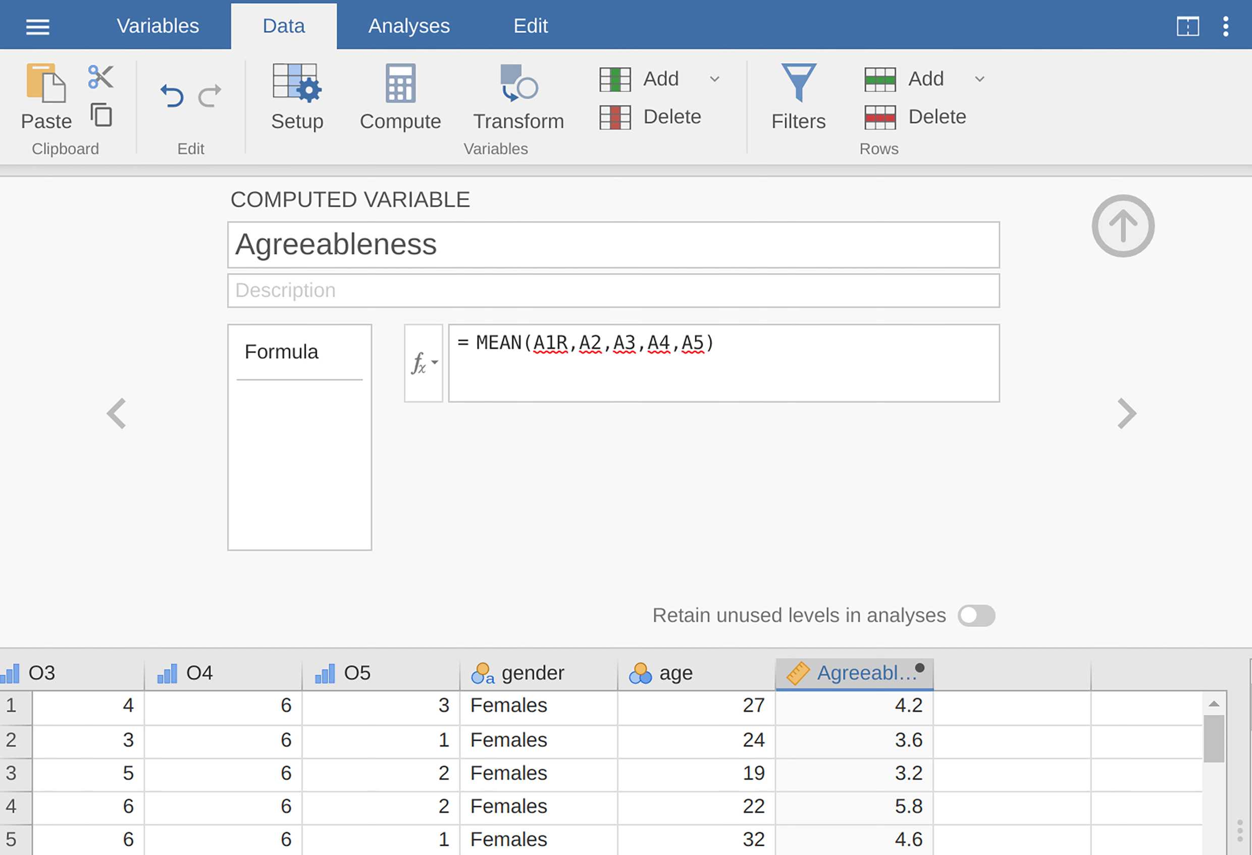
Fig. 203 Beregn en ny skalapoengvariabel ved hjelp av en beregnet variabel i jamovi

Another option is to create an optimally-weighted factor score index. To do this, save the factor scores to the data set, using the Factor scores checkbox in the drop-down menu Save. Once you have done this you will see that five new variables (columns) have been added to the data, one for each factor extracted (see Fig. 204 and Fig. 205).

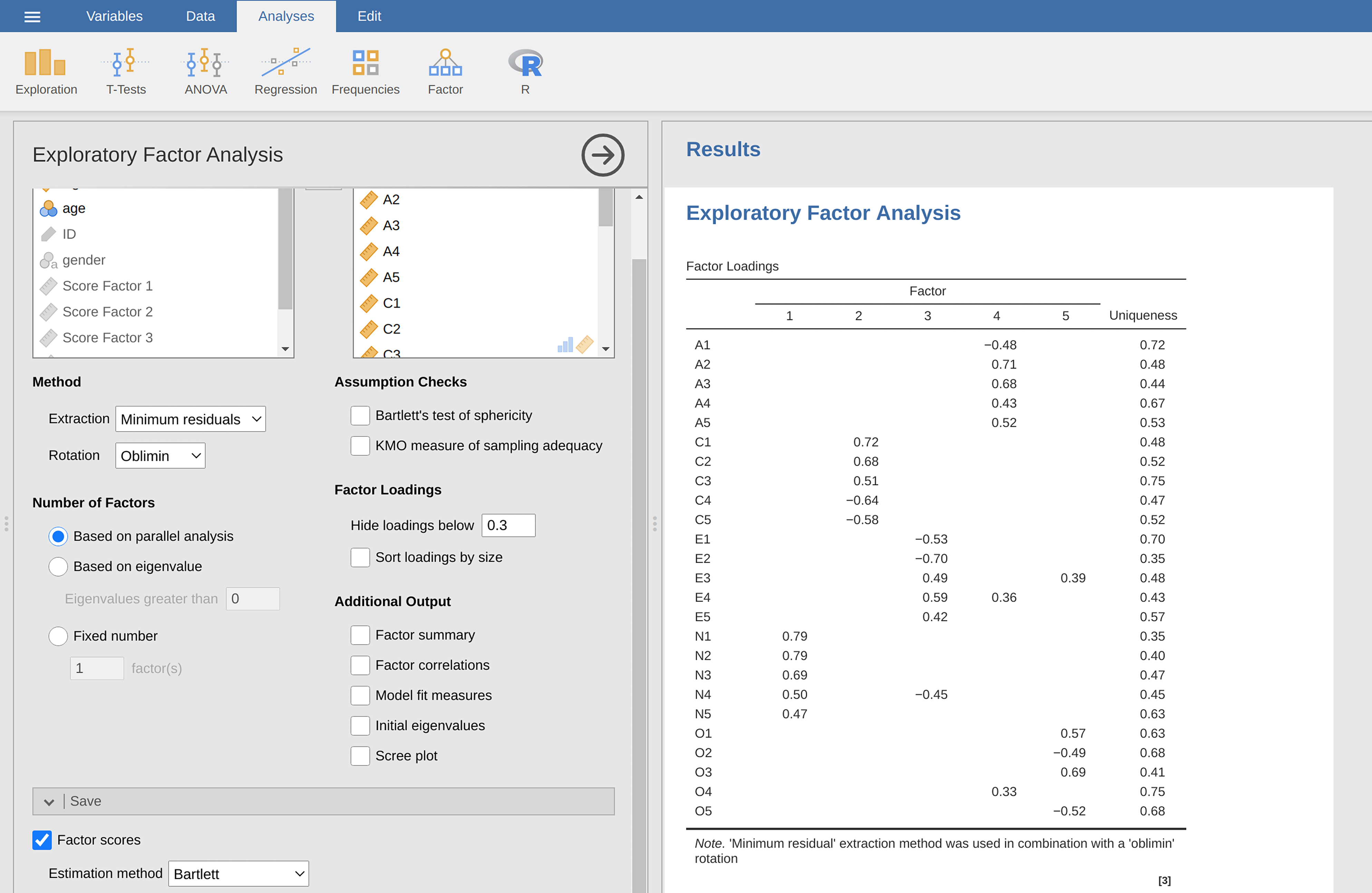
Fig. 204 Rj-editor-kommandoer for å lage optimalt vektede faktorskårer for femfaktorløsningen

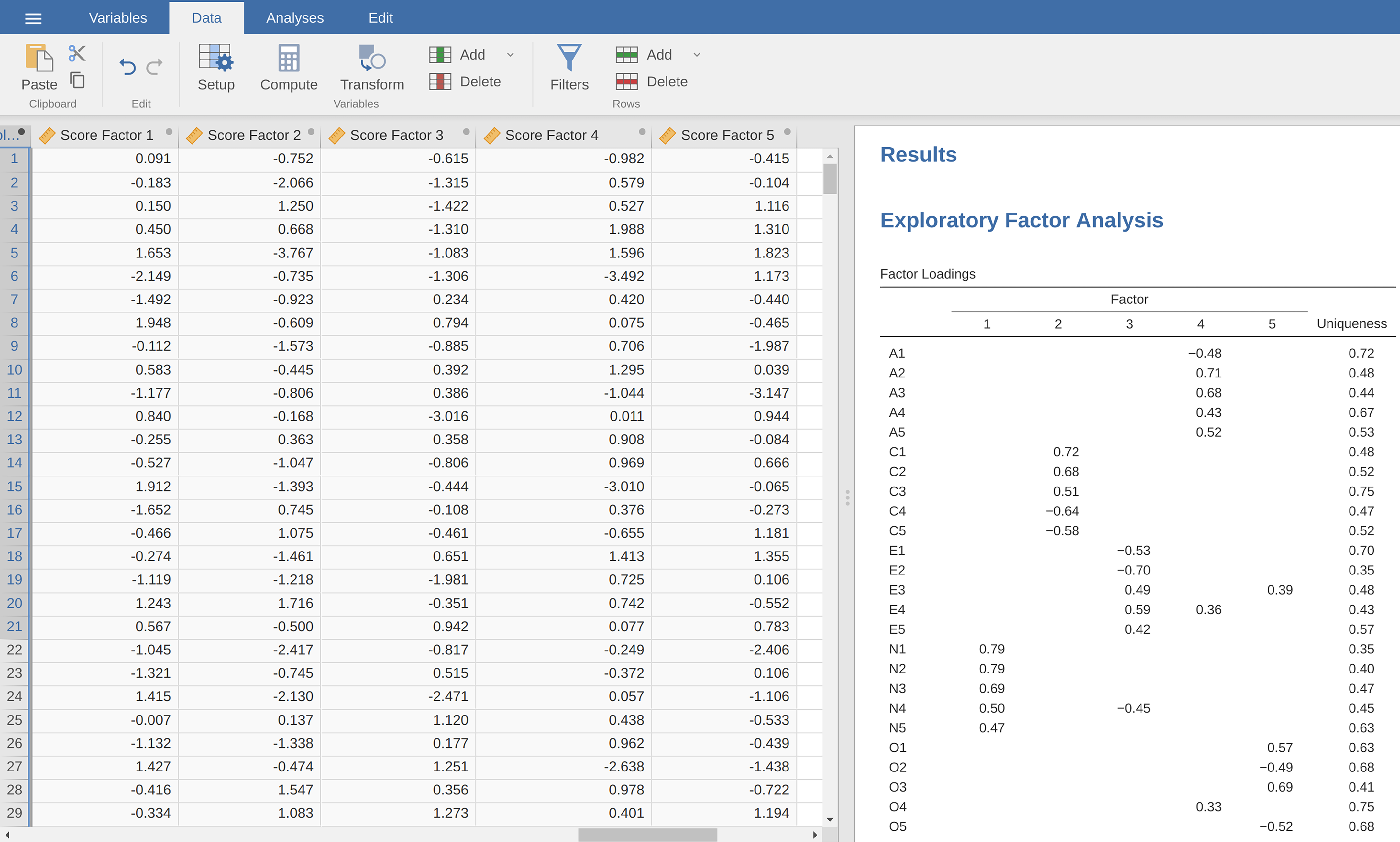
Fig. 205 Nyopprettet datafil bfifactscores.csv som er opprettet i Rj-editoren, og som inneholder de fem faktorskårvariablene. Legg merke til at hver av de nye faktorskårvariablene er merket i samme rekkefølge som faktorene er oppført i faktorladningstabellen.

Now you can go ahead and undertake further analyses, using either the factor- based scores (a mean scale score approach) or using the optimally-weighted factor scores calculated via the Rj editor. Your choice! For example, one thing you might like to do is see whether there are any gender differences in each of our personality scales. We did this for the Agreeableness score that we calculated using the factor-based score approach, and although the plot (see Fig. 206) showed that males were less agreeable than females, this was not a significant difference (Mann-Whitney U = 5760.5, p = 0.073).

Fig. 206 Sammenligning av forskjeller i Agreeableness-faktorbaserte skårer mellom menn og kvinner

Skriving av en EFA

Forhåpentligvis har vi så langt gitt deg en viss forståelse av EFA og hvordan man gjennomfører EFA i jamovi. Når du har gjennomført en EFA, hvordan skriver du den da? Det finnes ingen formell standard måte å skrive en EFA på, og eksemplene har en tendens til å variere etter fagfelt og forsker. Når det er sagt, finnes det likevel noen standardopplysninger som bør inkluderes i oppsummeringen:

1. Hva er det teoretiske grunnlaget for det området du studerer, og spesielt for de konstruktene du er interessert i å avdekke gjennom EFA?

2. A description of the sample (e.g., demographic information, sample size, sampling method).

3. En beskrivelse av hvilken type data som er brukt (f.eks. nominell , kontinuerlig ) og deskriptivstatistikk.

4. Beskriv hvordan du gikk frem for å teste forutsetningene for EFA. Detaljer om sfæricitetskontroller og mål på utvalgets tilstrekkelighet bør rapporteres.

5. Explain what FA extraction method (e.g., maximum likelihood) was used.

6. Forklar kriteriene og prosessen som ble brukt for å avgjøre hvor mange faktorer som ble trukket ut i den endelige løsningen, og hvilke spørsmål som ble valgt ut. Forklar tydelig begrunnelsen for viktige beslutninger under EFA-prosessen.

7. Forklar hvilke rotasjonsmetoder som ble forsøkt, hvorfor, og resultatene.

8. De endelige faktorladningene bør rapporteres i resultatene, i en tabell. Denne tabellen bør også rapportere unikheten (eller fellesskapet) for hver variabel (i den siste kolonnen). Faktorladningene bør rapporteres med beskrivende navner i tillegg til itemnumrene. Korrelasjoner mellom faktorene bør også inkluderes, enten nederst i denne tabellen eller i en separat tabell.

9. De ekstraherte faktorene bør gis meningsfulle navn. Det kan være lurt å bruke tidligere valgte faktornavn, men når du undersøker de faktiske spørsmålene og faktorene, kan det hende du mener at et annet navn er mer passende.

---

[1]

Faktorladningene kan tolkes som standardiserte regresjonskoeffisienter

[2]

A more advanced statistical technique, one which is beyond the scope of this book, undertakes regression modelling where latent factors are used in prediction models of other latent factors. This is called “structural equation modelling” and there are specific software programs and R packages dedicated to this approach.

[3]

An Eigen value indicates how much of the variance in the observed variables a factor accounts for. A factor with an Eigen value > 1 accounts for more variance than a single observed variable.

[4]

Oblique rotations provide two factor matrices, one called a structure matrix and one called a pattern matrix. In jamovi just the pattern matrix is shown in the results as this is typically the most useful for interpretation, though some experts suggest that both can be helpful. In a structure matrix coefficients show the relationship between the variable and the factors whilst ignoring the relationship of that factor with all the other factors (i.e., a zero-order correlation). Pattern matrix coefficients show the unique contribution of a factor to a variable whilst controlling for the effects of other factors on that variable (akin to standardized partial regression coefficient). Under orthogonal rotation, structure and pattern coefficients are the same.

[5]

Noen ganger rapporteres «kommunalitet» (communality) i faktoranalyse, som er hvor mye av variansen i en variabel som forklares av faktorløsningen. Unikhet er lik (1 - kommunalitet)

[6]

Husk å først reversere noen variabler hvis det er nødvendig.