Autor des Abschnitts: Danielle J. Navarro and David R. Foxcroft
Faktorielle ANOVA 3: unbalancierte Designs
Factorial ANOVA is a very handy thing to know about. It is been one of the standard tools used to analyse experimental data for many decades, and you will find that you can not read more than two or three papers in psychology without running into an ANOVA in there somewhere. However, there is one huge difference between the ANOVAs that you will see in a lot of real scientific articles and the ANOVAs that I have described so far. In in real life we are rarely lucky enough to have perfectly balanced designs. For one reason or another, it is typical to end up with more observations in some cells than in others. Or, to put it another way, we have an unbalanced design.
Unbalanced designs need to be treated with a lot more care than balanced designs, and the statistical theory that underpins them is a lot messier. It might be a consequence of this messiness, or it might be a shortage of time, but my experience has been that undergraduate research methods classes in psychology have a nasty tendency to ignore this issue completely. A lot of stats textbooks tend to gloss over it too. The net result of this, I think, is that a lot of active researchers in the field do not actually know that there is several different “types” of unbalanced ANOVAs, and they produce quite different answers. In fact, reading the psychological literature, I am kind of amazed at the fact that most people who report the results of an unbalanced factorial ANOVA do not actually give you enough details to reproduce the analysis. I secretly suspect that most people do not even realise that their statistical software package is making a whole lot of substantive data analysis decisions on their behalf. It is actually a little terrifying when you think about it. So, if you want to avoid handing control of your data analysis to stupid software, read on.
Der Kaffee-Datensatz
As usual, it will help us to work with some data. The coffee data set
contains a hypothetical data set that produces an unbalanced 3 × 2 ANOVA.
Suppose we were interested in finding out whether or not the tendency of people
to babble when they have too much coffee is purely an effect of the coffee
itself, or whether there is some effect of the milk and sugar that
people add to the coffee. Suppose we took 18 people and gave them some coffee
to drink. The amount of coffee, i.e., the caffeine, was held constant, and we
varied whether or not milk was added, so milk is a binary factor  with two levels,
 yes and no. We also varied the kind of sugar involved.
The coffee might contain real sugar or it might contain fake sugar
(i.e., artificial sweetener) or it might contain none at all, so the
sugar variable is a three level factor. Our outcome variable
babble is a continuous variable  that presumably refers to
some psychologically sensible measure of the extent to which someone is
“babbling”. The details do not really matter for our purpose. Take a look at
the data in the jamovi spreadsheet view, as in Abb. 191.
that presumably refers to
some psychologically sensible measure of the extent to which someone is
“babbling”. The details do not really matter for our purpose. Take a look at
the data in the jamovi spreadsheet view, as in Abb. 191.
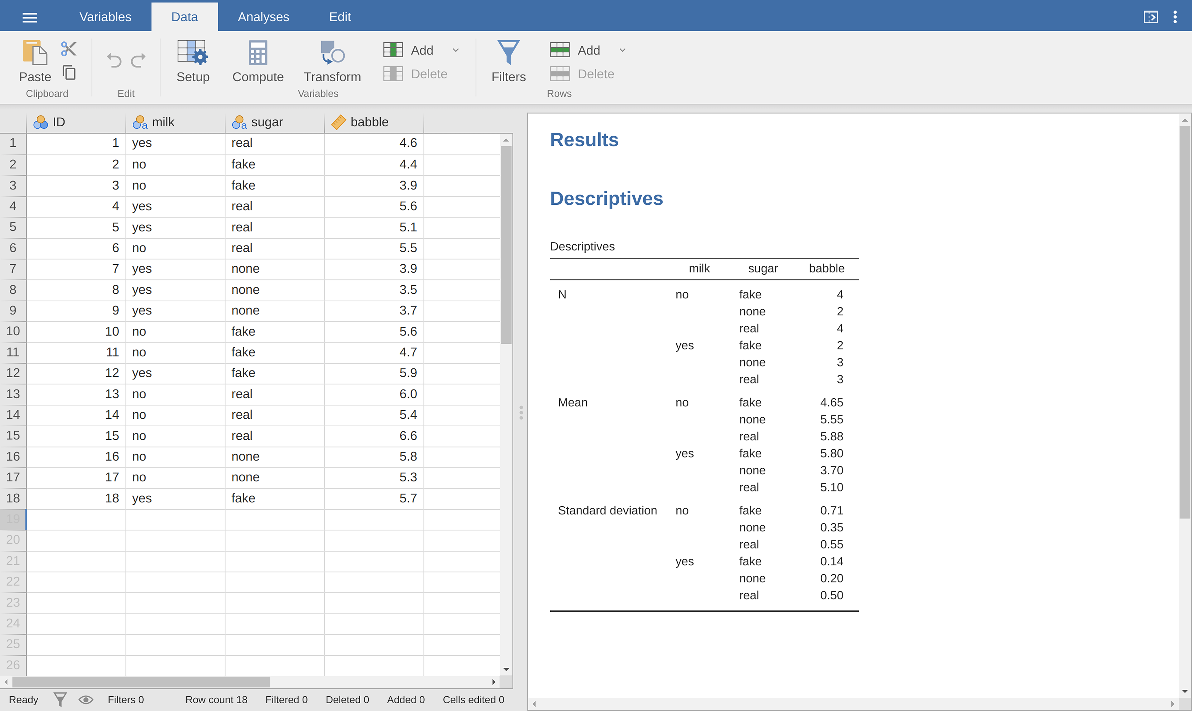
Abb. 191 Deskriptive Statistik für den coffee-Datensatz in jamovi, aggregiert nach den verschiedenen Ebenen der Faktoren sugar und milk
Looking at the table of means in Abb. 191 we get a strong impression
that there are differences between the groups. This is especially true when we
compare these means to the standard deviations for the babble variable.
Across groups, this standard deviation varies from 0.14 to 0.71, which is
fairly small relative to the differences in group means.[1] Whilst this at
first may seem like a straightforward factorial ANOVA, a problem arises when we
look at how many observations we have in each group. See the different Ns
for different groups shown in Abb. 191. This violates one of our
original assumptions, namely that the number of people in each group is the
same. We have not really discussed how to handle this situation.
Die „Standard-ANOVA“ existiert für unbalancierte Designs nicht
Unbalanced designs lead us to the somewhat unsettling discovery that there is not really any one thing that we might refer to as a standard ANOVA. In fact, it turns out that there are three fundamentally different ways[2] in which you might want to run an ANOVA in an unbalanced design. If you have a balanced design all three versions produce identical results, with the sums of squares, F-values, etc., all conforming to the formulas that I gave at the start of the chapter. However, when your design is unbalanced they do not give the same answers. Furthermore, they are not all equally appropriate to every situation. Some methods will be more appropriate to your situation than others. Given all this, it is important to understand what the different types of ANOVA are and how they differ from one another.
The first kind of ANOVA is conventionally referred to as Type 1 sum of
squares. I am sure you can guess what the other two are called. The “sum of
squares” part of the name was introduced by the SAS statistical software
package and has become standard nomenclature, but it is a bit misleading in
some ways. I think the logic for referring to them as different types of sum of
squares is that, when you look at the ANOVA tables that they produce, the key
difference in the numbers is the SS values. The degrees of freedom do not
change, the MS values are still defined as SS divided by df, etc.
However, what the terminology gets wrong is that it hides the reason why the
SS values are different from one another. To that end, it is a lot more
helpful to think of the three different kinds of ANOVA as three different
hypothesis testing strategies. These different strategies lead to different
SS values, to be sure, but it is the strategy that is the important thing
here, not the SS values themselves. Recall from section
Die ANOVA als lineares Modell, that any particular F-test is best thought of as a
comparison between two linear models. So, when you are looking at an ANOVA
table, it helps to remember that each of those F-tests corresponds to a
pair of models that are being compared. Of course, this leads naturally to
the question of which pair of models is being compared. This is the
fundamental difference between ANOVA Types 1, 2 and 3: each one corresponds to
a different way of choosing the model pairs for the tests. The Type 3 sum of
squares is the default method for hypothesis testing used by the ANOVA in
jamovi. To use another type of sum of squares, we have to select the respective
type in the Sum of squares selection box in the drop-down menu Model.
Typ-1-Quadratsumme
Die Methode vom Typ 1 wird manchmal auch als „sequentielle“ Quadratsumme bezeichnet, da sie einen Prozess beinhaltet, durch welchen dem Modell ein Term nach dem anderen hinzugefügt wird. Betrachten wir zum Beispiel die coffee-Daten. Nehmen wir an, wir wollen die vollständige 3 × 2 faktorielle ANOVA durchführen, einschließlich der Interaktionsterme. Das vollständige Modell enthält die Ergebnisvariable babble, die Prädiktorvariablen sugar und milk sowie den Interaktionsterm sugar * milk. Dies kann als babble ~ sugar + milk + sugar * milk geschrieben werden. Bei der Typ-1-Strategie wird dieses Modell sequentiell aufgebaut, wobei mit dem einfachsten möglichen Modell begonnen und nach und nach weitere Terme hinzugefügt werden.
The simplest possible model for the data would be one in which neither
milk nor sugar is assumed to have any effect on babbling. The only term
that would be included in such a model is the intercept, written as
babble ~ 1. This is our initial null hypothesis. The next simplest
model for the data would be one in which only one of the two main
effects is included. In the coffee data, there are two different
possible choices here, because we could choose to add milk first or to
add sugar first. The order actually turns out to matter, as we will see
later, but for now let us just make a choice arbitrarily and pick sugar.
So, the second model in our sequence of models is babble ~ sugar,
and it forms the alternative hypothesis for our first test. We now have
our first hypothesis test:
Nullmodell: |
|
Alternativmodell: |
|
Dieser Vergleich bildet unseren Hypothesentest für den Haupteffekt von sugar. Der nächste Schritt in unserer Modellbildung besteht darin, den anderen Haupteffekt-Term hinzuzufügen, so dass das nächste Modell in unserer Sequenz babble ~ sugar + milk ist. Der zweite Hypothesentest wird dann durch den Vergleich des folgenden Modellpaares gebildet:
Nullmodell: |
|
Alternativmodell: |
|
This comparison forms our hypothesis test of the main effect of
milk. In one sense, this approach is very elegant: the alternative
hypothesis from the first test forms the null hypothesis for the second
one. It is in this sense that the Type 1 method is strictly sequential.
Every test builds directly on the results of the last one. However, in
another sense it is very inelegant, because there is a strong asymmetry
between the two tests. The test of the main effect of sugar (the
first test) completely ignores milk, whereas the test of the main
effect of milk (the second test) does take sugar into account.
In any case, the fourth model in our sequence is now the full model,
babble ~ sugar + milk + sugar * milk, and the corresponding hypothesis
test is:
Nullmodell: |
|
Alternativmodell: |
|
Type 3 sum of squares is the default hypothesis testing method used by jamovi
ANOVA, so to run a Type 1 sum of squares analysis we have to select Type 1
in the Sum of squares selection box in the jamovi ANOVA → Model
options. This gives us the ANOVA table shown in Abb. 192.
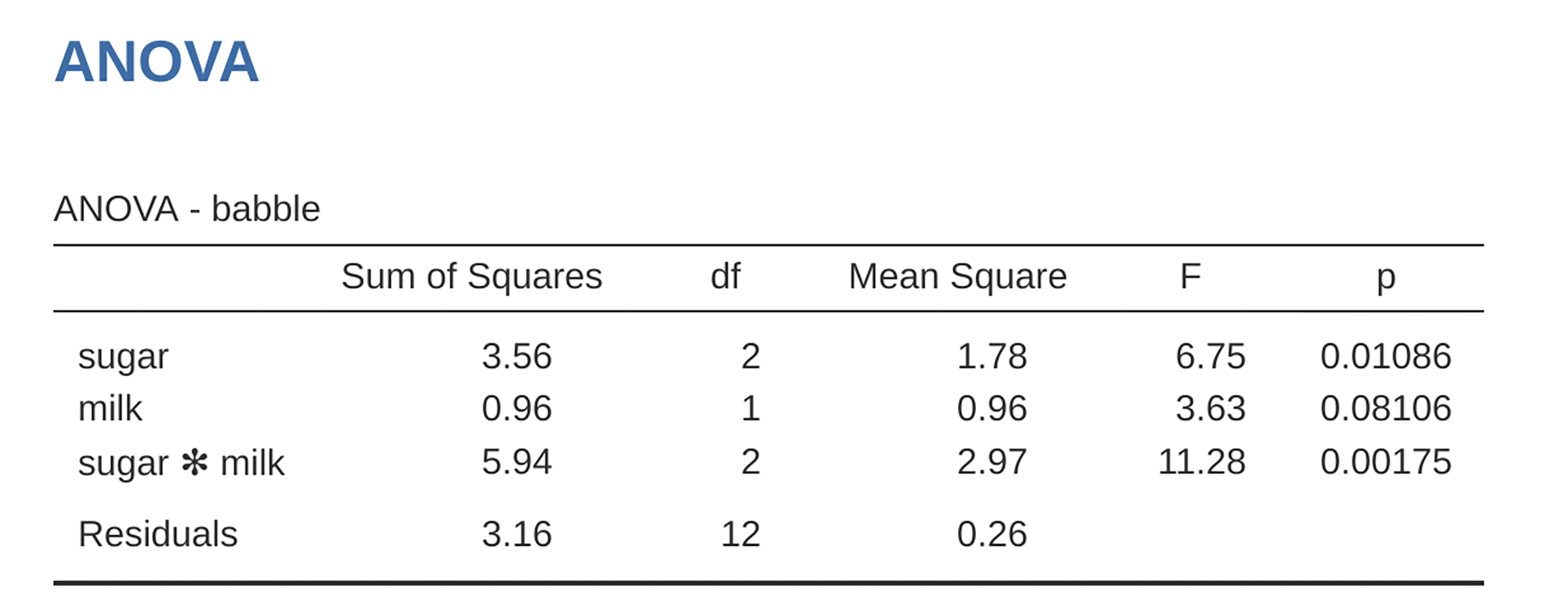
Abb. 192 ANOVA results table using Type 1 sum of squares in jamovi using the
coffee data set and a saturated model with the factors sugar,
milk, and their interaction (factor sugar is entered first)
The big problem with using Type 1 sum of squares is the fact that it really does depend on the order in which you enter the variables. Yet, in many situations the researcher has no reason to prefer one ordering over another. This is presumably the case for our milk and sugar problem. Should we add milk first or sugar first? It feels exactly as arbitrary as a data analysis question as it does as a coffee-making question. There may in fact be some people with firm opinions about ordering, but it is hard to imagine a principled answer to the question. Yet, look what happens when we change the ordering, as in Abb. 193.
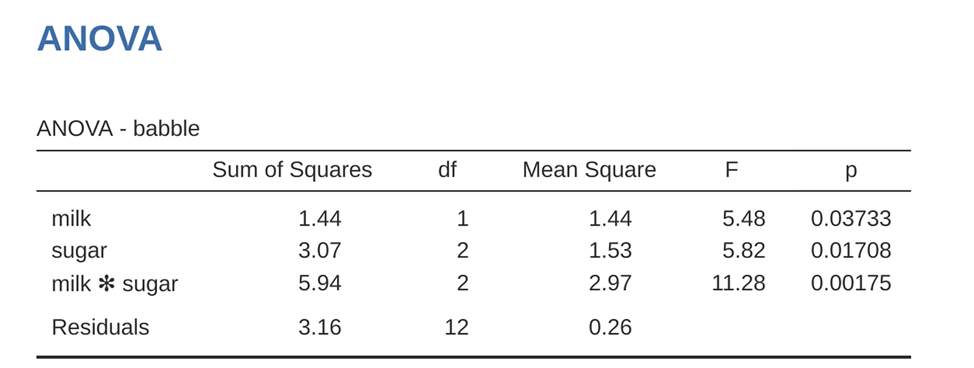
Abb. 193 ANOVA-Ergebnistabelle unter Verwendung von Typ-1-Quadratsumme in jamovi (mit dem coffee-Datensatz und einem gesättigten Modell mit den Faktoren sugar, milk, und deren Interaktion; der Faktor milk wurde zuerst hinzugefügt).
The p-values for both main effect terms have changed, and fairly
dramatically. Among other things, the effect of milk has become significant
(though one should avoid drawing any strong conclusions about this, as I have
mentioned previously). Which of these two ANOVAs should one report? It is not
immediately obvious.
When you look at the hypothesis tests that are used to define the “first” main
effect and the “second” one, it is clear that they are qualitatively different
from one another. In our initial example, we saw that the test for the main
effect of sugar completely ignores milk, whereas the test of the main
effect of milk does take sugar into account. As such, the Type 1
testing strategy really does treat the first main effect as if it had a kind of
theoretical primacy over the second one. In my experience there is very rarely
if ever any theoretically primacy of this kind that would justify treating any
two main effects asymmetrically.
Die Konsequenz aus all dem ist, dass Hypothesentests vom Typ 1 nur sehr selten von großem Interesse sind, so dass wir zu den Tests von Typ 2 und Typ 3 übergehen sollten.
Typ-3-Quadratsumme
Having just finished talking about Type 1 tests, you might think that the
natural thing to do next would be to talk about Type 2 tests. However, I think
it is actually a bit more natural to discuss Type 3 tests (which are simple and
the default in jamovi ANOVA) before talking about Type 2 tests (which are
trickier). The basic idea behind Type 3 tests is extremely simple. Regardless
of which term you are trying to evaluate, run the F-test in which the
alternative hypothesis corresponds to the full ANOVA model as specified by the
user, and the null model just deletes that one term that you are testing. For
instance, in the example from the coffee data set, in which our full model
was babble ~ sugar + milk + sugar * milk, the test for a main effect of
sugar would correspond to a comparison between the following two models:
Nullmodell: |
|
Alternativmodell: |
|
In ähnlicher Weise wird der Haupteffekt von milk getestet, indem das vollständige Modell mit einem Nullmodell verglichen wird, bei dem der Term milk entfernt wurde:
Nullmodell: |
|
Alternativmodell: |
|
Schließlich wird der Interaktionsterm sugar * milk auf genau die gleiche Weise ausgewertet. Auch hier testen wir das vollständige Modell gegen ein Nullmodell, bei dem der Interaktionsterm sugar * milk entfernt wurde:
Nullmodell: |
|
Alternativmodell: |
|
The basic idea generalises to higher order ANOVAs. For instance, suppose that
we were trying to run an ANOVA with three factors, A, B and C, and
we wanted to consider all possible main effects and all possible interactions,
including the three-way interaction A * B * C. The table below shows you
what the Type 3 tests look like for this situation:
Der geprüfte Term ist |
Das Nullmodell ist |
Das Alternativmodell ist |
|---|---|---|
|
|
|
|
|
|
|
|
|
|
|
|
|
|
|
|
|
|
|
|
|
As ugly as that table looks, it is pretty simple. In all cases, the alternative
hypothesis corresponds to the full model which contains three main effect terms
(e.g., A), three two-way interactions (e.g., A * B) and one three-way
interaction (i.e., A * B * C). The null model always contains six of these
seven terms, and the missing one is the one whose significance we are trying to
test.
At first pass, Type 3 tests seem like a nice idea. Firstly, we have removed the
asymmetry that caused us to have problems when running Type 1 tests. And
because we are now treating all terms the same way, the results of the
hypothesis tests do not depend on the order in which we specify them. This is
definitely a good thing. However, there is a big problem when interpreting the
results of the tests, especially for main effect terms. Consider the coffee
data. Suppose it turns out that the main effect of milk is not significant
according to the Type 3 tests. What this is telling us is that
babble ~ sugar + sugar * milk is a better model for the data than the full
model. But what does that even mean? If the interaction term sugar * milk
was also non-significant, we would be tempted to conclude that the data are
telling us that the only thing that matters is sugar. But suppose we have a
significant interaction term, but a non-significant main effect of milk. In
this case, are we to assume that there really is an “effect of sugar”, an
“interaction between milk and sugar”, but no “effect of milk”? That seems
crazy. The right answer simply must be that it is meaningless[3] to talk
about the main effect if the interaction is significant. In general, this seems
to be what most statisticians advise us to do, and I think that is the right
advice. But if it really is meaningless to talk about non-significant main
effects in the presence of a significant interaction, then it is not at all
obvious why Type 3 tests should allow the null hypothesis to rely on a model
that includes the interaction but omits one of the main effects that make it
up. When characterised in this fashion, the null hypotheses really do not make
much sense at all.
Later on, we will see that Type 3 tests can be redeemed in some contexts, but first let us take a look at the ANOVA results table using Type 3 sum of squares, see Abb. 194.
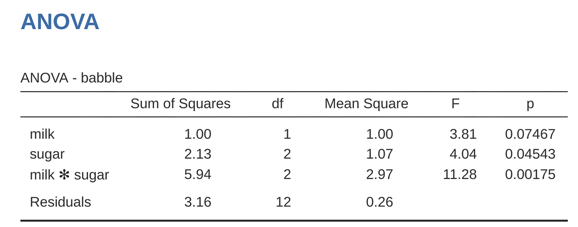
Abb. 194 ANOVA-Ergebnistabelle unter Verwendung von Typ-3-Quadratsumme in jamovi (mit dem coffee-Datensatz sowie einem gesättigten Modell mit den Faktoren sugar, milk und deren Interaktion).
But be aware, one of the perverse features of the Type 3 testing strategy is that typically the results turn out to depend on the contrasts that you use to encode your factors (see section Verschiedene Möglichkeiten, Kontraste zu definieren if you have forgotten what the different types of contrasts are).[4]
If the p-values that typically come out of Type 3 analyses (but not in jamovi) are so sensitive to the choice of contrasts, does that mean that Type 3 tests are essentially arbitrary and not to be trusted? To some extent that is true, and when we turn to a discussion of Type 2 tests we will see that Type 2 analyses avoid this arbitrariness entirely, but I think that is too strong a conclusion. Firstly, it is important to recognise that some choices of contrasts will always produce the same answers (ah, so this is what is happening in jamovi). Of particular importance is the fact that if the columns of our contrast matrix are all constrained to sum to zero, then the Type 3 analysis will always give the same answers.
Typ-2-Quadratsumme
Okay, so we have seen Type 1 and 3 tests now, and both are pretty straightforward. Type 1 tests are performed by gradually adding terms one at a time, whereas Type 3 tests are performed by taking the full model and looking to see what happens when you remove each term. However, both can have some limitations. Type 1 tests are dependent on the order in which you enter the terms, and Type 3 tests are dependent on how you code up your contrasts. Type 2 tests are a little harder to describe, but they avoid both of these problems, and as a result they are a little easier to interpret.
Type 2 tests are broadly similar to Type 3 tests. Start with a “full” model,
and test a particular term by deleting it from that model. However, Type 2
tests are based on the marginality principle which states that you should
not omit a lower order term from your model if there are any higher order ones
that depend on it. So, for instance, if your model contains the two-way
interaction A * B (a second order term), then it really ought to contain
the main effects A and B (first order terms). Similarly, if it contains
a three-way interaction term A * B * C, then the model must also include
the main effects A, B and C as well as the simpler interactions
A * B, A * C and B * C. Type 3 tests routinely violate the
marginality principle. For instance, consider the test of the main effect of
A in the context of a three-way ANOVA that includes all possible
interaction terms. According to Type 3 tests, our null and alternative models
are:
Nullmodell: |
|
Alternativmodell: |
|
Beachten Sie, dass die Nullhypothese A auslässt, aber A * B, A * C und A * B * C als Teil des Modells einschließt. Nach den Tests vom Typ 2 ist dies keine gute Wahl der Nullhypothese. Wenn wir stattdessen die Nullhypothese testen wollen, dass A für unser outcome nicht relevant ist, sollten wir die Nullhypothese angeben, die das komplizierteste Modell ist, das sich nicht auf A in irgendeiner Form stützt, auch nicht als Interaktion. Die Alternativhypothese entspricht diesem Nullmodell plus einem Haupteffektterm von A. Dies ist viel näher an dem, was die meisten Leute intuitiv als „Haupteffekt von A“ ansehen würden, und es ergibt sich das Folgende als unser Typ-2-Test des Haupteffekts von A:[5]
Nullmodell: |
|
Alternativmodell: |
|
Anyway, just to give you a sense of how the Type 2 tests play out, see the full table of tests that would be applied in a three-way factorial ANOVA:
Der geprüfte Term ist |
Das Nullmodell ist |
Das Alternativmodell ist |
|---|---|---|
|
|
|
|
|
|
|
|
|
|
|
|
|
|
|
|
|
|
|
|
|
In the context of the two-way ANOVA that we have been using in the coffee
data, the hypothesis tests are even simpler. The main effect of sugar
corresponds to an F-test comparing these two models:
Nullmodell: |
|
Alternativmodell: |
|
The test for the main effect of milk is:
Nullmodell: |
|
Alternativmodell: |
|
Schließlich lautet der Test für die Interaktion sugar * milk:
Nullmodell: |
|
Alternativmodell: |
|
Running the tests are again straightforward. Just select Type 2 in the
Sum of squares selection box in the jamovi ANOVA → Model options,
This gives us the ANOVA table shown in Abb. 195.
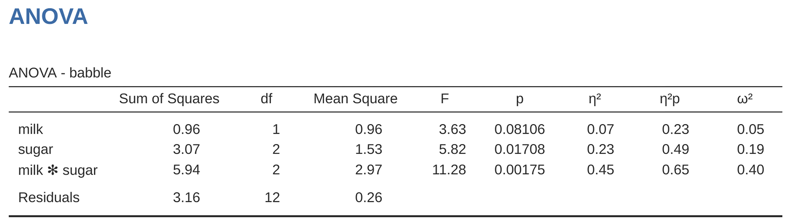
Abb. 195 ANOVA-Ergebnistabelle unter Verwendung von Typ-2-Quadratsumme in jamovi (mit dem coffee-Datensatz sowie einem gesättigten Modell mit den Faktoren sugar, milk und deren Interaktion).
Type 2 tests have some clear advantages over Type 1 and Type 3 tests. They do not depend on the order in which you specify factors (unlike Type 1), and they do not depend on the contrasts that you use to specify your factors (unlike Type 3). And although opinions may differ on this last point, and it will definitely depend on what you are trying to do with your data, I do think that the hypothesis tests that they specify are more likely to correspond to something that you actually care about. As a consequence, I find that it is usually easier to interpret the results of a Type 2 test than the results of a Type 1 or Type 3 test. For this reason my tentative advice is that, if you can not think of any obvious model comparisons that directly map onto your research questions but you still want to run an ANOVA in an unbalanced design, Type 2 tests are probably a better choice than Type 1 or Type 3.[6]
Effektstärken (und nicht-additive Quadratsummen)
jamovi also provides the effect sizes η² and partial η² when you select these options, as in Abb. 195. However, when you have got an unbalanced design there is a bit of extra complexity involved.
If you remember back to our very early discussions of ANOVA, one of the key ideas behind the sums of squares calculations is that if we add up all the SS terms associated with the effects in the model, and add that to the residual SS, they are supposed to add up to the total sum of squares. And, on top of that, the whole idea behind η² is that, because you are dividing one of the SS terms by the total SS value, an η² value can be interpreted as the proportion of variance accounted for by a particular term. But this is not so straightforward in unbalanced designs because some of the variance goes “missing”.
This seems a bit odd at first, but here is why. When you have unbalanced designs your factors become correlated with one another, and it becomes difficult to tell the difference between the effect of factor A and the effect of factor B. In the extreme case, suppose that we would run a 2 × 2 design in which the number of participants in each group had been as follows:
Zucker |
kein Zucker |
|
|---|---|---|
Milch |
100 |
0 |
keine Milch |
0 |
100 |
Here we have a spectacularly unbalanced design: 100 people have milk and sugar, 100 people have no milk and no sugar, and that is all. There are 0 people with milk and no sugar, and 0 people with sugar but no milk. Now suppose that, when we collected the data, it turned out there is a large (and statistically significant) difference between the “milk and sugar” group and the “no-milk and no-sugar” group. Is this a main effect of sugar? A main effect of milk? Or an interaction? It is impossible to tell, because the presence of sugar has a perfect association with the presence of milk. Now suppose the design had been a little more balanced:
Zucker |
kein Zucker |
|
|---|---|---|
Milch |
100 |
5 |
keine Milch |
5 |
100 |
This time around, it is technically possible to distinguish between the effect of milk and the effect of sugar, because we have a few people that have one but not the other. However, it will still be pretty difficult to do so, because the association between sugar and milk is still extremely strong, and there are so few observations in two of the groups. Again, we are very likely to be in the situation where we know that the predictor variables (milk and sugar) are related to the outcome (babbling), but we do not know if the nature of that relationship is a main effect of one or the other predictor, or the interaction.
This uncertainty is the reason for the missing variance. The “missing” variance corresponds to variation in the outcome variable that is clearly attributable to the predictors, but we do not know which of the effects in the model is responsible. When you calculate Type 1 sum of squares, no variance ever goes missing. The sequential nature of Type 1 sum of squares means that the ANOVA automatically attributes this variance to whichever effects are entered first. However, the Type 2 and Type 3 tests are more conservative. Variance that cannot be clearly attributed to a specific effect does not get attributed to any of them, and it goes missing.