Autor des Abschnitts: Danielle J. Navarro and David R. Foxcroft

Teststatistiken und Stichprobenverteilungen

At this point we need to start talking specifics about how a hypothesis test is constructed. To that end, let us return to the ESP example. Let us ignore the actual data that we obtained, for the moment, and think about the structure of the experiment. Regardless of what the actual numbers are, the form of the data is that X out of N people correctly identified the colour of the hidden card. Moreover, let us suppose for the moment that the null hypothesis really is true, that ESP does not exist and the true probability that anyone picks the correct colour is exactly θ = 0.5. What would we expect the data to look like? Well, obviously we would expect the proportion of people who make the correct response to be pretty close to 50%. Or, to phrase this in more mathematical terms, we would say that X / N is approximately 0.5. Of course, we would not expect this fraction to be exactly 0.5. If, for example, we tested N = 100 people and X = 53 of them got the question right, we would probably be forced to concede that the data are quite consistent with the null hypothesis. On the other hand, if X = 99 of our participants got the question right then we would feel pretty confident that the null hypothesis is wrong. Similarly, if only X = 3 people got the answer right we would be similarly confident that the null hypothesis was wrong. Let us be a little more technical about this. We have a quantity X that we can calculate by looking at our data. After looking at the value of X we make a decision about whether to believe that the null hypothesis is correct, or to reject the null hypothesis in favour of the alternative. The name for this thing that we calculate to guide our choices is a test statistic.

Nachdem wir eine Teststatistik ausgewählt haben, besteht der nächste Schritt darin, genau anzugeben, welche Werte der Teststatistik dazu führen würden, dass wir die Nullhypothese ablehnen, und welche Werte dazu führen würden, dass wir sie beibehalten müssen. Dazu müssen wir bestimmen, wie die Stichprobenverteilung der Teststatistik aussehen würde, wenn die Nullhypothese tatsächlich wahr wäre (über Stichprobenverteilungen haben wir bereits in Stichprobenverteilung des Mittelwertes gesprochen). Warum brauchen wir das? Weil diese Verteilung uns genau sagt, welche Werte von X unsere Nullhypothese erwarten lassen würde. Und deshalb können wir diese Verteilung als Hilfsmittel verwenden, um zu beurteilen, wie gut die Nullhypothese mit unseren Daten übereinstimmt.

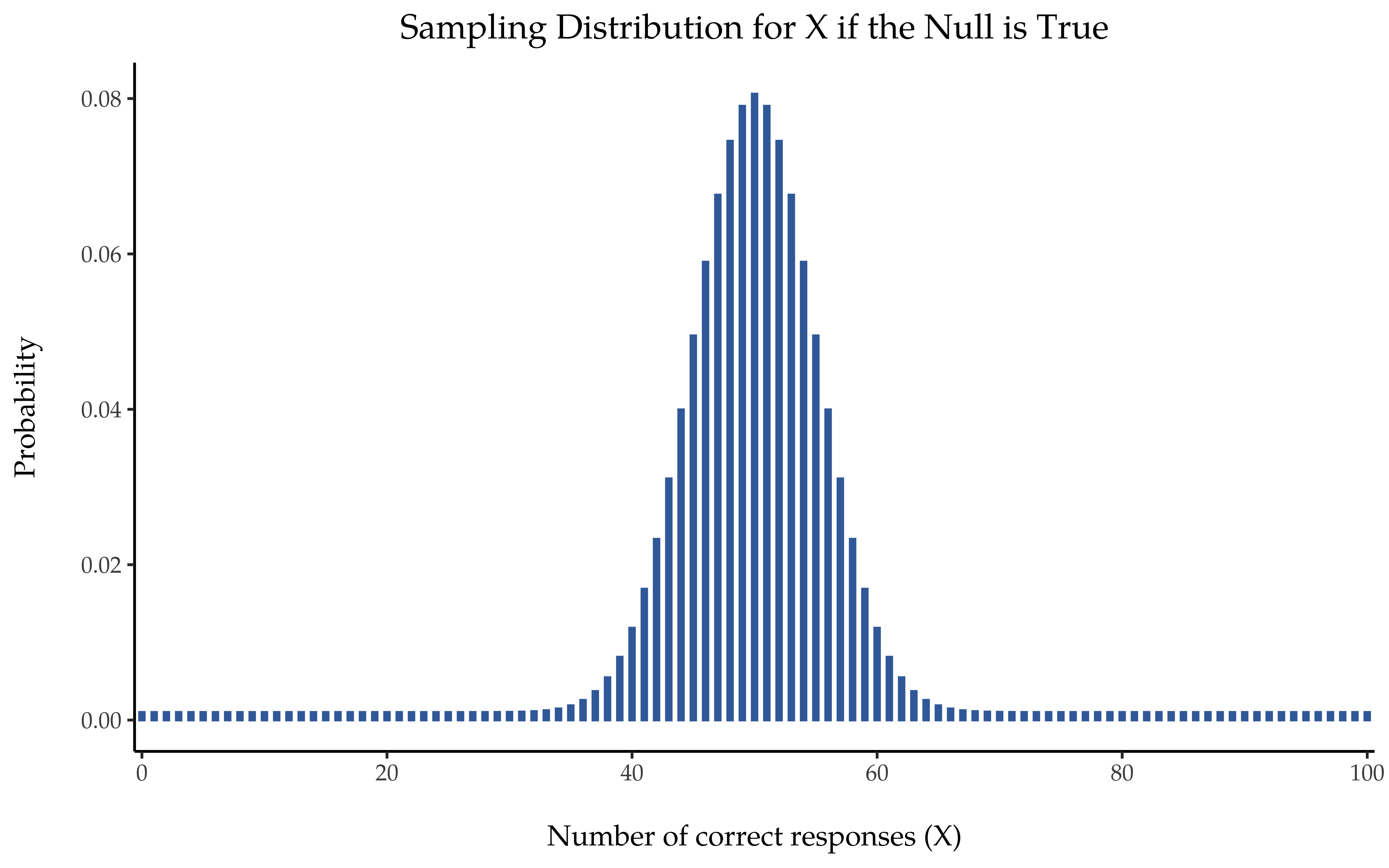
Abb. 81 Die Stichprobenverteilung für unsere Teststatistik X, wenn die Nullhypothese wahr ist. Für unser ESP-Szenario ist dies eine Binomialverteilung. Da die Nullhypothese besagt, dass die Wahrscheinlichkeit einer richtigen Antwort θ = 0,5 ist, überrascht es uns kaum, dass der wahrscheinlichste Wert in unserer Stichprobenverteilung bei 50 (von 100) richtigen Antworten liegt. Der Anteil der Antworten mit der höchsten Wahrscheinlichkeitsdichte liegt zwischen 40 und 60.

How do we actually determine the sampling distribution of the test statistic? For a lot of hypothesis tests this step is actually quite complicated, and later on in the book you will see me being slightly evasive about it for some of the tests (some of them I do not even understand myself). However, sometimes it is very easy. And, fortunately for us, our ESP example provides us with one of the easiest cases. Our population parameter θ is just the overall probability that people respond correctly when asked the question, and our test statistic X is the count of the number of people who did so out of a sample size of N. We have seen a distribution like this before, in section Die Binomialverteilung, and that is exactly what the binomial distribution describes! So, to use the notation and terminology that I introduced in that section, we would say that the null hypothesis predicts that X is binomially distributed, which is written:

X ~ Binomial(θ, N)

Since the null hypothesis states that θ = 0.5 and our experiment has N = 100 people, we have the sampling distribution we need. This sampling distribution is plotted in Abb. 81. No surprises really, the null hypothesis says that X = 50 is the most likely outcome, and it says that we are almost certain to see somewhere between 40 and 60 correct responses.