Autor des Abschnitts: Danielle J. Navarro and David R. Foxcroft
Schätzen eines Konfidenzintervalls
Statistics means never having to say you are certain—Unbekannte Herkunft[1]
Up to this point in this chapter, I have outlined the basics of sampling theory which statisticians rely on to make guesses about population parameters on the basis of a sample of data. As this discussion illustrates, one of the reasons we need all this sampling theory is that every data set leaves us with some uncertainty, so our estimates are never going to be perfectly accurate. The thing that has been missing from this discussion is an attempt to quantify the amount of uncertainty that attaches to our estimate. It is not enough to be able guess that, say, the mean IQ of undergraduate psychology students is 115 (yes, I just made that number up). We also want to be able to say something that expresses the degree of certainty that we have in our guess. For example, it would be nice to be able to say that there is a 95% chance that the true mean lies between 109 and 121. The name for this is a confidence interval for the mean.
Armed with an understanding of sampling distributions, constructing a confidence interval for the mean is actually pretty easy. Here is how it works. Suppose the true population mean is µ and the standard deviation is σ. I have just finished running my study that has N participants, and the mean IQ among those participants is X̄. We know from our discussion of the central limit theorem that the sampling distribution of the mean is approximately normal. We also know from our discussion of the normal distribution, that there is a 95% chance that a normally-distributed quantity will fall within about two standard deviations of the true mean.
To be more precise, the more correct answer is that there is a 95% chance that a normally-distributed quantity will fall within 1.96 standard deviations of the true mean. Next, recall that the standard deviation of the sampling distribution is referred to as the standard error, and the standard error of the mean is written as SEM. When we put all these pieces together, we learn that there is a 95% probability that the sample mean X̄ that we have actually observed lies within 1.96 standard errors of the population mean.
Mathematisch lässt sich dies wie folgt ausdrücken:
where the SEM is equal to \(\sigma / \sqrt{$N$}\) and we can be 95% confident that this is true. However, that is not answering the question that we are actually interested in. The equation above tells us what we should expect about the sample mean given that we know what the population parameters are. What we want is to have this work the other way around. We want to know what we should believe about the population parameters, given that we have observed a particular sample. However, it is not too difficult to do this. Using a little high school algebra, a sneaky way to rewrite our equation is like this:
Das bedeutet, dass der Wertebereich mit einer Wahrscheinlichkeit von 95 % den Mittelwert der Grundgesamtheit µ enthält. Wir bezeichnen diesen Bereich als 95%-Konfidenzintervall, bezeichnet als KI95 (oder CI95). Kurz gesagt, solange N hinreichend groß ist (groß genug, um zu glauben, dass die Stichprobenverteilung des Mittelwerts normal ist), können wir dies als unsere Formel für das 95%-Konfidenzintervall schreiben:
Of course, there is nothing special about the number 1.96. It just happens to be the multiplier you need to use if you want a 95% confidence interval. If I had wanted a 70% confidence interval, I would have used 1.04 as the magic number rather than 1.96.
Ein kleiner Fehler in der Formel
As usual, I lied. The formula that I have given above for the 95% confidence interval is approximately correct, but I glossed over an important detail in the discussion. Notice my formula requires you to use the standard error of the mean, SEM, which in turn requires you to use the true population standard deviation σ. Yet, in Schätzen von Populationsparametern I stressed the fact that we do not actually know the true population parameters. Because we do not know the true value of σ we have to use an estimate of the population standard deviation \(\hat{\sigma}\) instead. This is pretty straightforward to do, but this has the consequence that we need to use the percentiles of the t-distribution rather than the normal distribution to calculate our magic number, and the answer depends on the sample size. When N is very large, we get pretty much the same value using the t-distribution or the normal distribution: 1.96. But when N is small we get a much bigger number when we use the t-distribution: 2.26.
There is nothing too mysterious about what is happening here. Bigger values mean that the confidence interval is wider, indicating that we are more uncertain about what the true value of µ actually is. When we use the t-distribution instead of the normal distribution we get bigger numbers, indicating that we have more uncertainty. And why do we have that extra uncertainty? Well, because our estimate of the population standard deviation \(\hat\sigma\) might be wrong! If it is wrong, it implies that we are a bit less sure about what our sampling distribution of the mean actually looks like, and this uncertainty ends up getting reflected in a wider confidence interval.
Interpretieren eines Konfidenzintervalls
The hardest thing about confidence intervals is understanding what they mean. Whenever people first encounter confidence intervals, the first instinct is almost always to say that “there is a 95% probability that the true mean lies inside the confidence interval”. It is simple and it seems to capture the common sense idea of what it means to say that I am “95% confident”. Unfortunately, it is not quite right. The intuitive definition relies very heavily on your own personal beliefs about the value of the population mean. I say that I am 95% confident because those are my beliefs. In everyday life that is perfectly okay, but if you remember back to Was bedeutet Wahrscheinlichkeit?, you will notice that talking about personal belief and confidence is a Bayesian idea. However, confidence intervals are not Bayesian tools. Like everything else in this chapter, confidence intervals are frequentist tools, and if you are going to use frequentist methods then it is not appropriate to attach a Bayesian interpretation to them. If you use frequentist methods, you must adopt frequentist interpretations!
Okay, so if that is not the right answer, what is? Remember what we said about frequentist probability. The only way we are allowed to make “probability statements” is to talk about a sequence of events, and to count up the frequencies of different kinds of events. From that perspective, the nterpretation of a 95% confidence interval must have something to do with replication. Specifically, if we replicated the experiment over and over again and computed a 95% confidence interval for each replication, then 95% of those intervals would contain the true mean. More generally, 95% of all confidence intervals constructed using this procedure should contain the true population mean. This idea is illustrated in Abb. 80, which shows 50 confidence intervals constructed for a “measure 10 IQ scores” experiment (top panel) and another 50 confidence intervals for a “measure 25 IQ scores” experiment (bottom panel). A bit fortuitously, across the 100 replications that I simulated, it turned out that exactly 95 of them contained the true mean.
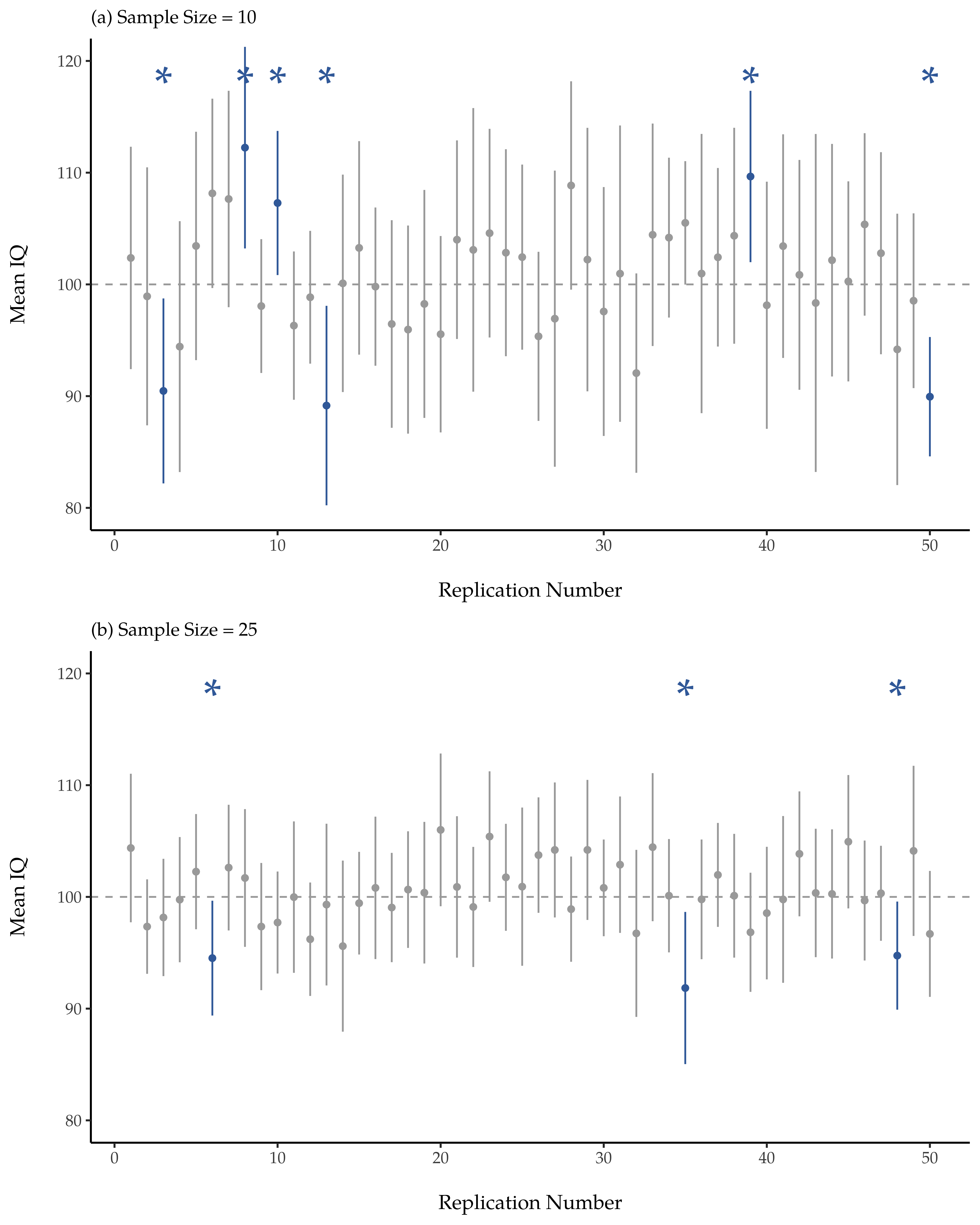
Abb. 80 95%-Konfidenzintervalle. Die obere Abbildung zeigt 50 simulierte Wiederholungen eines Experiments, bei dem wir den IQ von 10 Personen messen. Der Punkt markiert die Position des Stichprobenmittelwerts und die Linie zeigt das 95%-Konfidenzintervall. Insgesamt enthalten 47 der 50 Konfidenzintervalle den wahren Mittelwert (d. h. 100), die drei mit Sternchen markierten Intervalle jedoch nicht. Die untere Abbildung zeigt eine ähnliche Simulation, aber dieses Mal simulieren wir Wiederholungen eines Experiments, bei dem der IQ von 25 Personen gemessen wird.
The critical difference here is that the Bayesian claim makes a probability statement about the population mean (i.e., it refers to our uncertainty about the population mean), which is not allowed under the frequentist interpretation of probability because you can not “replicate” a population! In the frequentist claim, the population mean is fixed and no probabilistic claims can be made about it. Confidence intervals, however, are repeatable so we can replicate experiments. Therefore a frequentist is allowed to talk about the probability that the confidence interval (a random variable) contains the true mean, but is not allowed to talk about the probability that the true population mean (not a repeatable event) falls within the confidence interval.
I know that this seems a little pedantic, but it does matter. It matters because the difference in interpretation leads to a difference in the mathematics. There is a Bayesian alternative to confidence intervals, known as credible intervals. In most situations credible intervals are quite similar to confidence intervals, but in other cases they are drastically different. As promised, though, I will talk more about the Bayesian perspective in chapter Bayessche Statistik.
Berechnung von Konfidenzintervallen in jamovi
jamovi bietet eine einfache Möglichkeit zur Berechnung von Konfidenzintervallen für den Mittelwert als Teil der Funktionalität von Descriptives. Setzen Sie dort einfach die Checkbox Confidence interval for Mean.
95% confidence intervals are the de facto standard in psychology. So, for
example, if I load the IQsim data set (our simulated large sample data with
N = 10 000), and check Confidence interval for Mean under
Descriptives, we obtain a mean IQ score of 99.683 with a 95% CI from
99.391 to 99.975.
When it comes to plotting confidence intervals for the mean in jamovi, this is
not (yet) available as part of the Descriptives options. However, when we
get onto learning about specific statistical tests, for example in chapter
Vergleich mehrerer Mittelwerte (einfaktorielle ANOVA), we will see that we can plot confidence intervals
as part of the data analysis. That is pretty cool, so we will show you how to
do that later on.