Afsnitsforfatter: Danielle J. Navarro and David R. Foxcroft

Basic probability theory

Ideological arguments between Bayesians and frequentists notwithstanding, it turns out that people mostly agree on the rules that probabilities should obey. There are lots of different ways of arriving at these rules. The most commonly used approach is based on the work of Andrey Kolmogorov, one of the great Soviet mathematicians of the 20th century. I will not go into a lot of detail, but I will try to give you a bit of a sense of how it works. And in order to do so I am going to have to talk about my trousers.

Introducing probability distributions

One of the disturbing truths about my life is that I only own five pairs of trousers. Even sadder, I have given them names: I call them X₁, X₂, X₃, X₄ and X₅. If I were to describe this situation using the language of probability theory, I would refer to each pair of trousers (i.e., each X) as an elementary event. The key characteristic of elementary events is that every time we make an observation (e.g., every time I put on a pair of trousers) then the outcome will be one and only one of these events. Like I said, these days I always wear exactly one pair of trousers so my trousers satisfy this constraint. Similarly, the set of all possible events is called a sample space. Granted, some people would call it a “wardrobe”, but that is because they are refusing to think about my trousers in probabilistic terms.

Now that we have a sample space (a wardrobe), which is built from lots of possible elementary events (trousers), what we want to do is assign a probability of one of these elementary events. For an event X, the probability of that event P(X) is a number that lies between 0 and 1. The bigger the value of P(X), the more likely the event is to occur. So, for example, if P(X) = 0 it means the event X is impossible (i.e., I never wear those trousers). On the other hand, if P(X) = 1 it means that event X is certain to occur (i.e., I always wear those trousers). For probability values in the middle it means that I sometimes wear those trousers. For instance, if P(X) = 0.5 it means that I wear those trousers half of the time.

At this point, we are almost done. The last thing we need to recognise is that “something always happens”. Every time I put on trousers, I really do end up wearing trousers. What this somewhat trite statement means, in probabilistic terms, is that the probabilities of the elementary events need to add up to 1. This is known as the law of total probability, not that any of us really care. More importantly, if these requirements are satisfied then what we have is a probability distribution. For example, this is an example of a probability distribution:

Which trousers?	Label	Probability
Blue jeans	X1	P(X1) = 0.5
Grey jeans	X2	P(X2) = 0.3
Black jeans	X3	P(X3) = 0.1
Black suit	X4	P(X4) = 0
Blue tracksuit	X5	P(X5) = 0.1

Each of the events has a probability that lies between 0 and 1, and if we add up the probability of all events they sum to 1. We can even draw a nice bar graph (see Bar graphs) to visualise this distribution, as shown in figur 58.

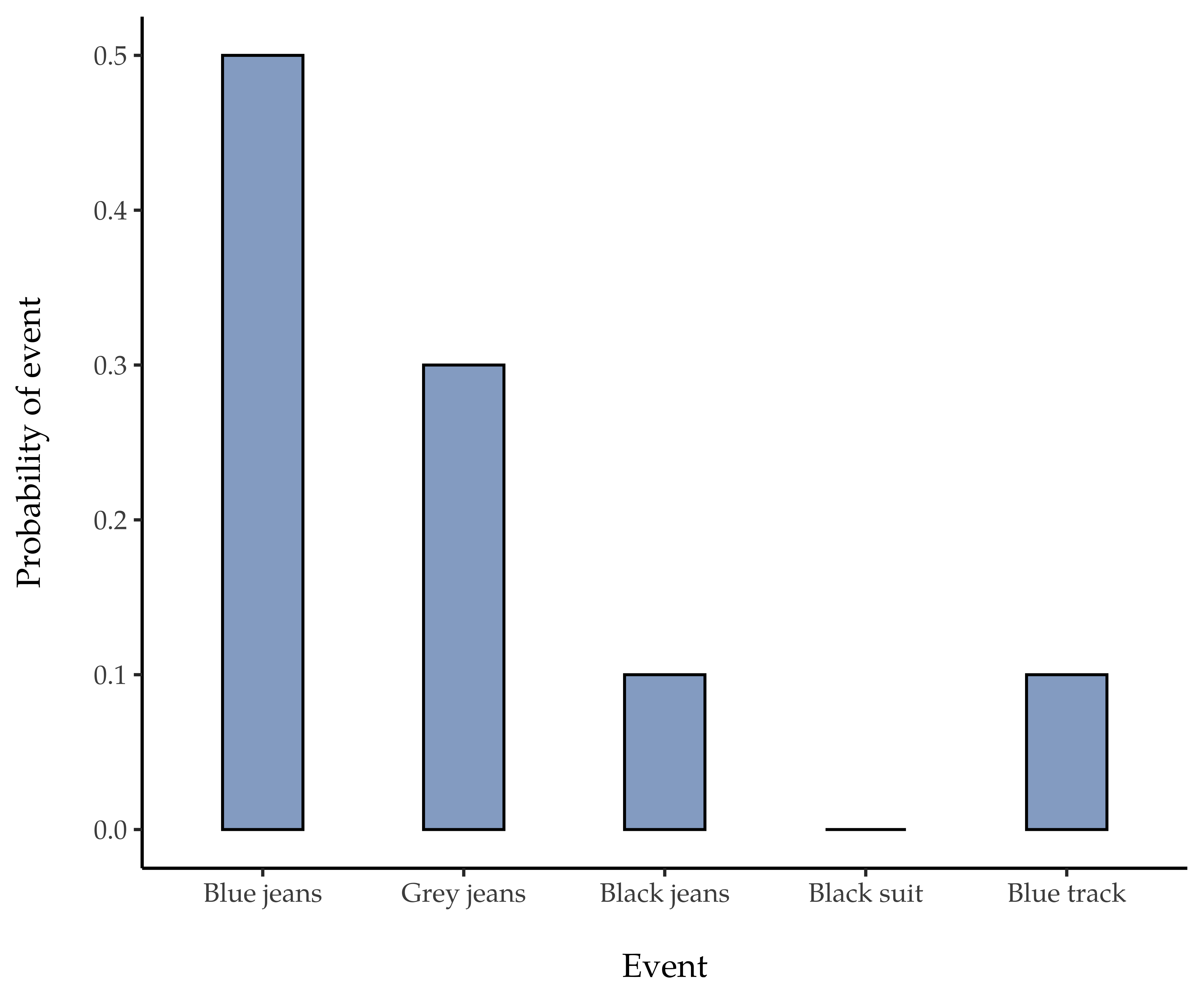
figur 58 Visual depiction of the “trousers” probability distribution. There are five “elementary events”, corresponding to the five pairs of trousers that I own. Each event has some probability of occurring: this probability is a number between 0 to 1. The sum of these probabilities is 1.

And, at this point, we have all achieved something. You have learned what a probability distribution is, and I have finally managed to find a way to create a graph that focuses entirely on my trousers. Everyone wins! The only other thing that I need to point out is that probability theory allows you to talk about non-elementary events as well as elementary ones. The easiest way to illustrate the concept is with an example. In the trousers example it is perfectly legitimate to refer to the probability that I wear jeans. In this scenario, the “Danielle wears jeans” event is said to have happened as long as the elementary event that actually did occur is one of the appropriate ones. In this case “blue jeans”, “black jeans” or “grey jeans”. In mathematical terms, we defined the “jeans” event E to correspond to the set of elementary events (X₁, X₂, X₃)`. If any of these elementary events occurs then E is also said to have occurred. Having decided to write down the definition of the E this way, it is pretty straightforward to state what the probability P(E) is: we just add everything up. In this particular case:

P(E) = P(X₁) + P(X₂) + P(X₃)

Since the probabilities of blue, grey and black jeans respectively are 0.5, 0.3 and 0.1, the probability that I wear jeans is equal to 0.9.

You might be thinking that this is all terribly obvious and simple and you would be right. All we have really done is wrap some basic mathematics around a few common sense intuitions. However, from these simple beginnings it is possible to construct some extremely powerful mathematical tools. I am definitely not going to go into the details in this book, but what I will do is list, in tabel 6, some of the other rules that probabilities satisfy. These rules can be derived from the simple assumptions that I have outlined above, but since we do not actually use these rules for anything in this book I will not do so here.

tabel 6 Some basic rules that probabilities must satisfy. You do not really need to know these rules in order to understand the analyses that we will talk about later in the book, but they are important if you want to understand probability theory a bit more deeply.

English	Notation		Formula
not A	P(¬ A)	=	1 - P(A)
A or B	P(A ∪ B)	=	P(A) + P(B) - P(A ∩ B)
A and B	P(A ∩ B)	=	P(A|B) P(B)