Afsnitsforfatter: Danielle J. Navarro and David R. Foxcroft
The binomial distribution
As you might imagine, probability distributions vary enormously and there is an enormous range of distributions out there. However, they are not all equally important. In fact, the vast majority of the content in this book relies on one of five distributions: the binomial distribution, the normal distribution, the t-distribution, the χ²-distribution (chi-square) and the F-distribution. Given this, what I will do over the next few sections is provide a brief introduction to all five of these, paying special attention to the binomial and the normal. I will start with the binomial distribution since it is the simplest of the five.
Introducing the binomial
The theory of probability originated in the attempt to describe how games of chance work, so it seems fitting that our discussion of the binomial distribution should involve a discussion of rolling dice and flipping coins. Let us imagine a simple “experiment”. In my hot little hand I am holding 20 identical six-sided dice. On one face of each die there is a picture of a skull, the other five faces are all blank. If I proceed to roll all 20 dice, what is the probability that I will get exactly four skulls? Assuming that the dice are fair, we know that the chance of any one dice coming up skulls is 1 in 6. To say this another way, the skull probability for a single dice is approximately 0.167. This is enough information to answer our question, so let us have a look at how it is done.
Binomial |
Normal |
|---|---|
\(P(X \ | \ \theta, N) = \displaystyle\frac{N!}{X! (N - X)!} \theta ^ X (1 - \theta) ^ {N - X}\) |
\(p(X \ | \ \mu, \sigma) = \displaystyle\frac{1}{\sqrt{2 \pi} \sigma} \exp \left( -\frac{(X - \mu) ^ 2}{2 \sigma ^ 2} \right)\) |
As usual, we will want to introduce some names and some notation. We will let N denote the number of dice rolls in our experiment, which is often referred to as the size parameter of our binomial distribution. We will also use θ to refer to the the probability that a single dice comes up skulls, a quantity that is usually called the success probability of the binomial.[1] Finally, we will use X to refer to the results of our experiment, namely the number of skulls I get when I roll the dice. Since the actual value of X is due to chance we refer to it as a random variable. In any case, now that we have all this terminology and notation we can use it to state the problem a little more precisely. The quantity that we want to calculate is the probability that X = 4 given that we know that θ = 0.167 and N = 20. The general “form” of the thing I am interested in calculating could be written as:
P(X | θ, N)
and we are interested in the special case where X = 4, θ = 0.167 and N = 20. There is only one more piece of notation I want to refer to before moving on to discuss the solution to the problem. If I want to say that X is generated randomly from a binomial distribution with parameters θ and N, the notation I would use is as follows:
X ~ Binomial(θ, N)
I know what you are thinking: notation, notation, notation. Really, who cares? Very few readers of this book are here for the notation, so I should probably move on and talk about how to use the binomial distribution. I have included the formula for the binomial distribution in tabel 7, since some readers may want to play with it themselves, but since most people probably do not care that much and because we do not need the formula in this book, I will not talk about it in any detail. Instead, I just want to show you what the binomial distribution looks like.
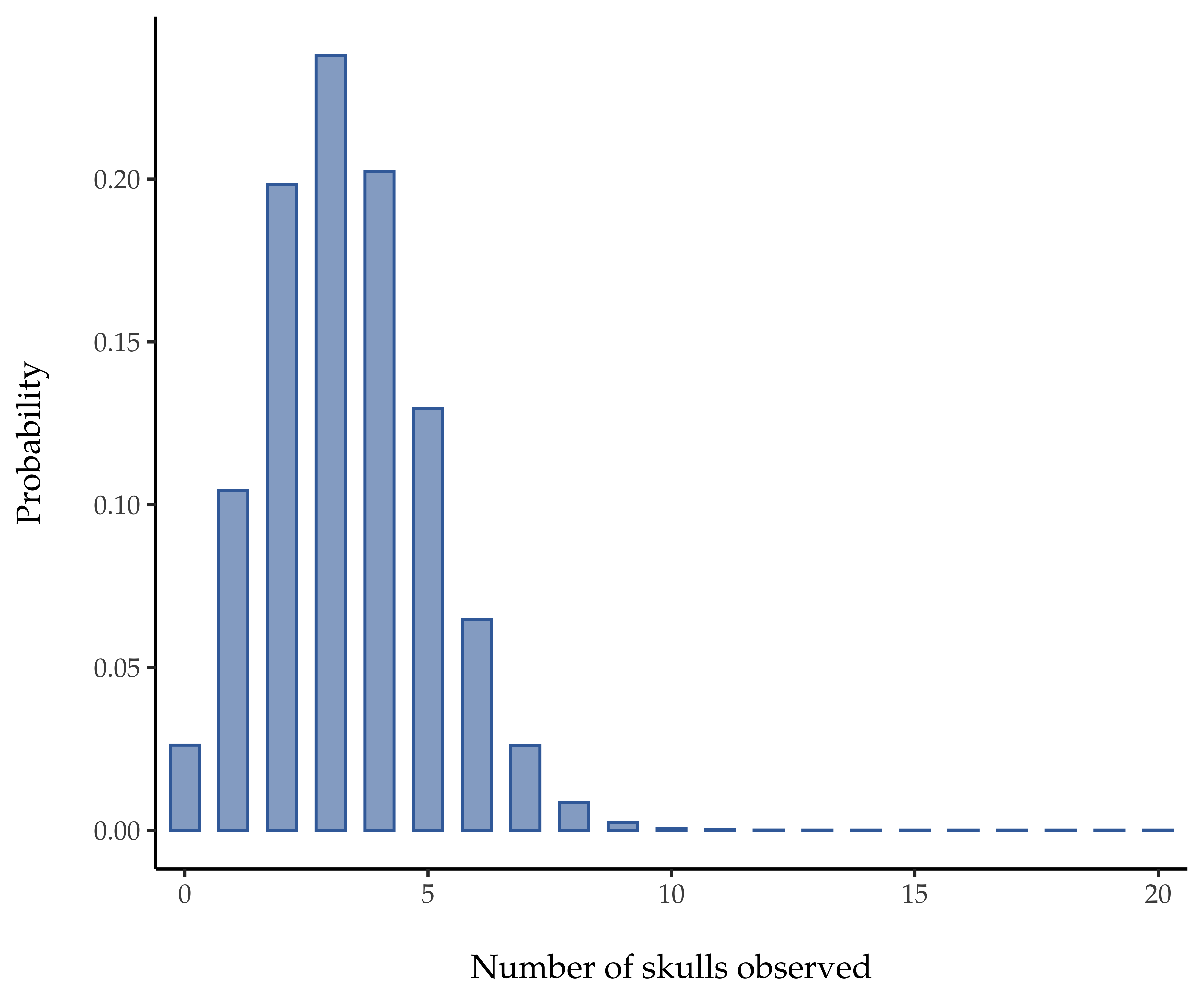
figur 59 Binomial distribution with size parameter of N = 20 and an underlying success probability of θ = 1/6. Each vertical bar depicts the probability of one specific outcome (i.e., one possible value of X). Because this is a probability distribution, each of the probabilities must be a number between 0 and 1, and the heights of the bars must sum to 1 as well.
To that end, figur 59 plots the binomial probabilities for all possible values of X for our dice rolling experiment, from X = 0 (no skulls) all the way up to X = 20 (all skulls). Note that this is basically a bar chart, and is no different to the “trousers probability” plot I drew in figur 58. On the horizontal axis we have all the possible events, and on the vertical axis we can read off the probability of each of those events. So, the probability of rolling four skulls out of 20 is about 0.20 (the actual answer is 0.2022036, as we will see in a moment). In other words, you would expect that to happen about 20% of the times you repeated this experiment.
To give you a feel for how the binomial distribution changes when we alter the values of θ and N, let us suppose that instead of rolling dice I am actually flipping coins. This time around, my experiment involves flipping a fair coin repeatedly and the outcome that I am interested in is the number of heads that I observe. In this scenario, the success probability is now θ = 1/2. Suppose I were to flip the coin N = 20 times. In this example, I have changed the success probability but kept the size of the experiment the same. What does this do to our binomial distribution? Well, as the left panel of figur 60 shows, the main effect of this is to shift the whole distribution, as you would expect. Okay, what if we flipped a coin N = 100 times? Well, in that case we get what is shown in the right panel. The distribution stays roughly in the middle but there is a bit more variability in the possible outcomes.
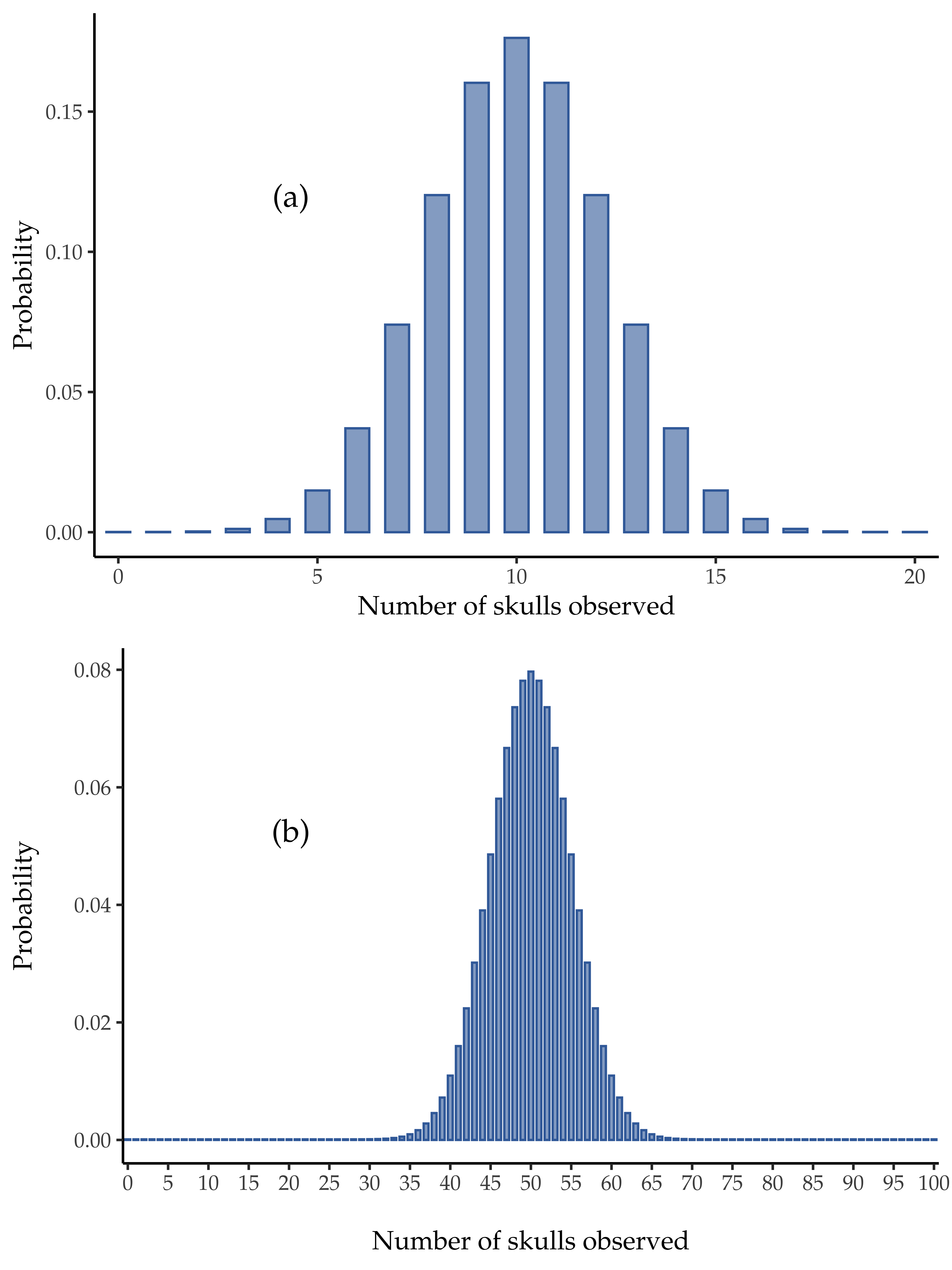
figur 60 Two binomial distributions, involving a scenario in which I am flipping a fair coin, so the underlying success probability is θ = 1/2. In the left panel, we assume I am flipping the coin N = 20 times. In the right panel, we assume that the coin is flipped N = 100 times.