Forfatter av avsnitt: Danielle J. Navarro and David R. Foxcroft
Enveis ANOVA for gjentatte målinger
Enveis ANOVA for gjentatte målinger er en statistisk metode for å teste for signifikante forskjeller mellom tre eller flere grupper der de samme deltakerne brukes i hver gruppe (eller der hver deltaker er tett matchet med deltakere i andre eksperimentgrupper). Av denne grunn bør det alltid være like mange poengsummer (datapunkter) i hver forsøksgruppe. Denne typen design og analyse kan også kalles en «relatert ANOVA» eller en «within-subjects ANOVA».
The logic behind a repeated measures ANOVA is very similar to that of an independent ANOVA (sometimes called a “between-subjects” ANOVA). You will remember that earlier we showed that in a between-subjects ANOVA total variability is partitioned into between-groups variability (SSb) and within-groups variability (SSw), then divided by their respective degrees of freedom to give MSb and MSw (see Table 16), whereupon the F-ratio is calculated as:
In a repeated measures ANOVA, the F-ratio is calculated in a similar way, but whereas in an independent ANOVA the within-group variability (SSw) is used as the basis for the MSw denominator, in a repeated measures ANOVA the SSw is partioned into two parts. As we are using the same subjects in each group, we can remove the variability due to the individual differences between subjects (referred to as SSsubjects) from the within-groups variability. We will not go into too much technical detail about how this is done, but essentially each subject becomes a level of a factor called subjects. The variability in this within-subjects factor is then calculated in the same way as any between-subjects factor. And then we can subtract SSsubjects from SSw to provide a smaller SSerror term:
This change in SSerror term often leads to a more powerful statistical test, but this does depend on whether the reduction in the SSerror more than compensates for the reduction in degrees of freedom for the error term: the degrees of freedom go from (n - k)[1] to (n - 1)(k - 1) remembering that there are more subjects in the independent ANOVA design.
ANOVA for gjentatte målinger i jamovi
Først trenger vi noen data. Geschwind (1972) har foreslått at den nøyaktige karakteren av en pasients språkvansker etter et hjerneslag kan brukes til å diagnostisere den spesifikke regionen i hjernen som har blitt skadet. En forsker er opptatt av å identifisere de spesifikke kommunikasjonsvanskene hos seks pasienter som lider av Brocas afasi (en språkvanske som ofte oppstår etter et hjerneslag).
Deltaker |
Tale |
Konseptuell |
Syntaks |
|---|---|---|---|
1 |
8 |
7 |
6 |
2 |
7 |
8 |
6 |
3 |
9 |
5 |
3 |
4 |
5 |
4 |
5 |
5 |
6 |
6 |
2 |
6 |
8 |
7 |
4 |
Pasientene måtte gjennomføre tre ordgjenkjenningsoppgaver. I den første oppgaven (taleproduksjon) skulle pasientene gjenta enkeltord som ble lest høyt av forskeren. I den andre oppgaven (begrepsforståelse), som skulle teste ordforståelsen, skulle pasientene matche en rekke bilder med riktig navn. I den tredje oppgaven (syntaks), som skulle teste kunnskap om korrekt ordstilling, ble pasientene bedt om å omorganisere syntaktisk ukorrekte setninger. Hver pasient fullførte alle tre oppgavene. Rekkefølgen pasientene løste oppgavene i, ble utjevnet mellom deltakerne. Hver oppgave besto av en serie på 10 forsøk. Antall forsøk som ble fullført av hver pasient, vises i Table 17. Legg inn disse dataene i jamovi klar for analyse (eller ta en snarvei og last inn datasettet broca).
To perform a one-way related ANOVA in jamovi, open the one-way repeated
measures ANOVA dialogue box, as in Fig. 160, via ANOVA → Repeated
Measures ANOVA. Then:
Skriv inn et navn for
Repeated Measures Factors(opprinnelig:RM Factor…). Dette bør være en etikett som du velger for å beskrive forholdene som gjentas av alle deltakerne. For eksempel, for å beskrive tale-, begreps- og syntaksoppgavene som ble fullført av alle deltakerne, vil en passende etikett væreTask. Merk at dette nye faktornavnet representerer den uavhengige variabelen i analysen.Legg til et tredje nivå i variabelboksen
Repeated Measures Factors, siden det er tre nivåer som representerer de tre oppgavene:Speech,ConceptualogSyntax. Endre etikettene på nivåene tilsvarende.Flytt deretter hver av nivåvariablene over til tekstboksen
Repeated Measures Cells.Til slutt krysser du av for
Sphericity checksunder alternativetAssumption Checks.
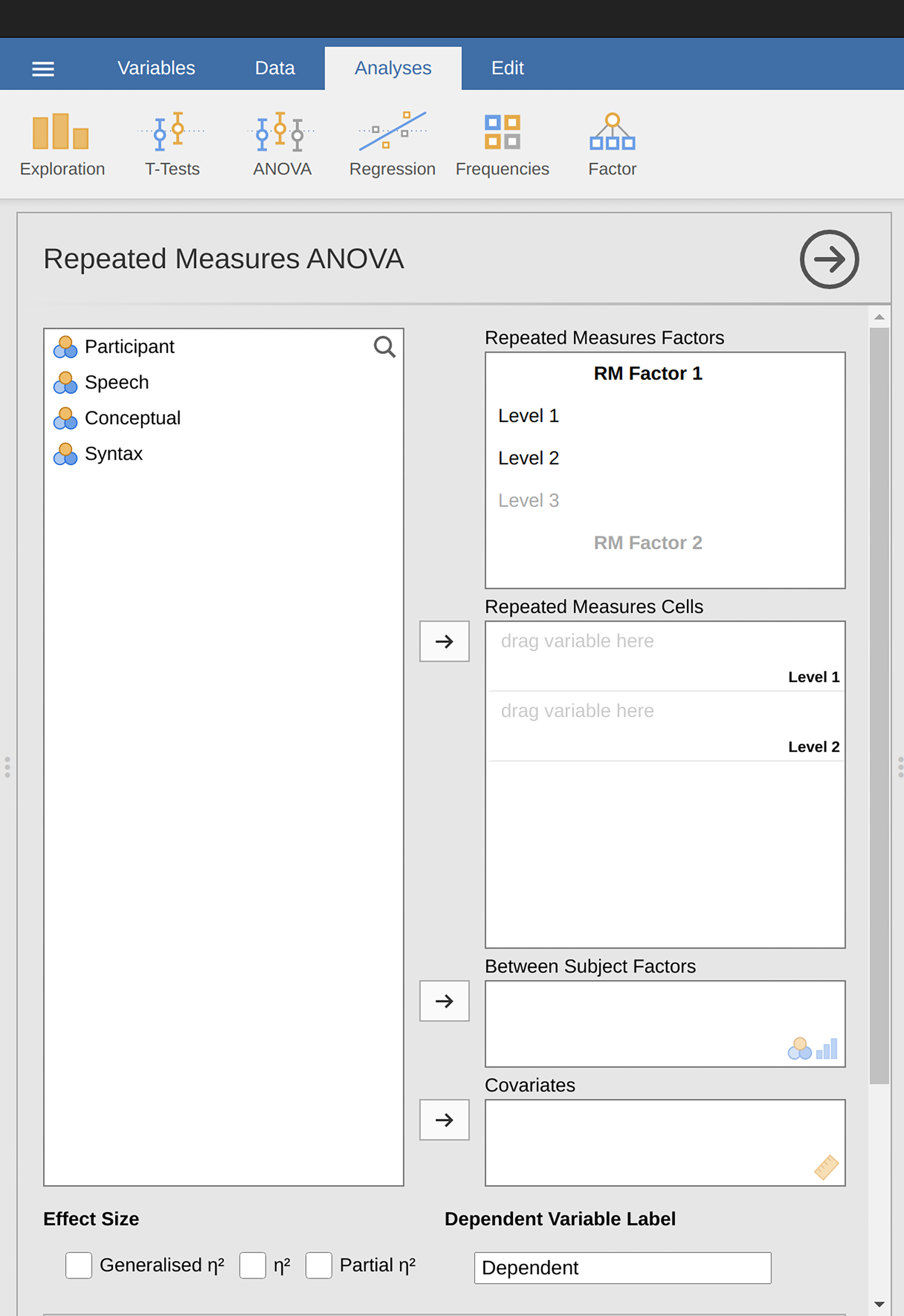
Fig. 160 Dialogboks for ANOVA for gjentatte målinger i jamovi
jamovi output for a one-way Repeated Measures ANOVA is produced as shown
in the Fig. 161 to Fig. 164. The first output we should
look at is Mauchly’s Test of Sphericity, which tests the hypothesis that
the variances of the differences between the conditions are equal (meaning that
the spread of difference scores between the study conditions is approximately
the same). In Fig. 161, Mauchly’s test significance level is p =
0.720. If Mauchly’s test is non-significant (i.e., p > 0.05, as is the case
in this analysis) then it is reasonable to conclude that the variances of the
differences are not significantly different (i.e., they are roughly equal and
sphericity can be assumed).
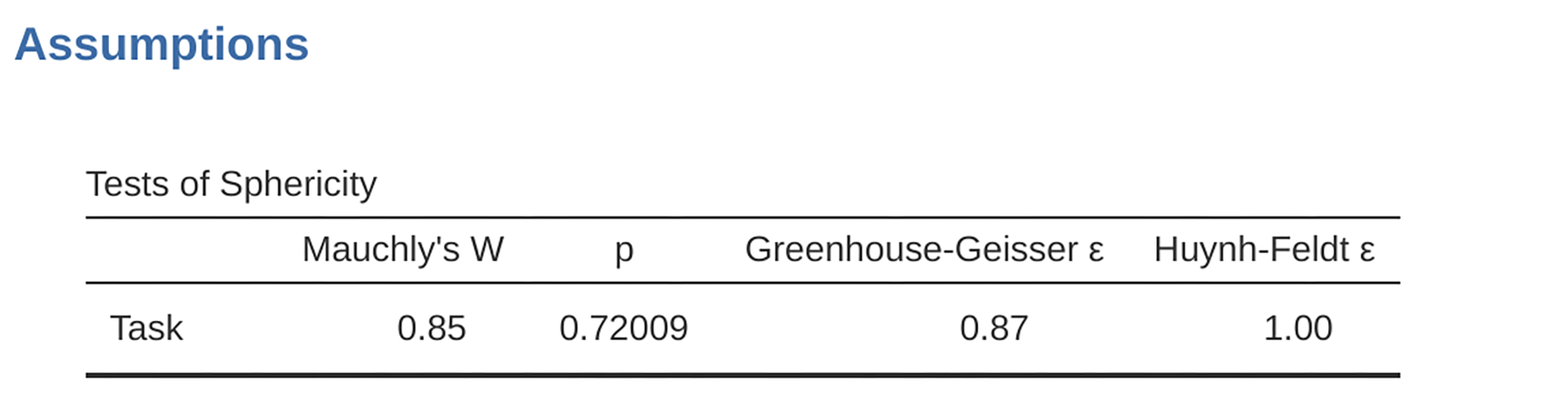
Fig. 161 Enveis ANOVA for gjentatte målinger: Mauchlys test av sfæricitet
Hvis Mauchlys test derimot hadde vært signifikant (p < 0,05), ville vi konkludert med at det er signifikante forskjeller mellom variansen i forskjellene, og at kravet om sfæricitet ikke er oppfylt. I dette tilfellet bør vi korrigere F-verdien som ble oppnådd i den enveisrelaterte ANOVA-analysen:
If the
Greenhouse-Geisser εvalue in theTests of Sphericitytable is > 0.75 then you should use the Huynh-Feldt correction.But if the
Greenhouse-Geisser εvalue is < 0.75, then you should use the Greenhouse-Geisser correction.
Both these corrected F-values can be specified in the Sphericity
Corrections check boxes under the Assumption Checks options, and the
corrected F-values are then shown in the results table, as in
Fig. 162.
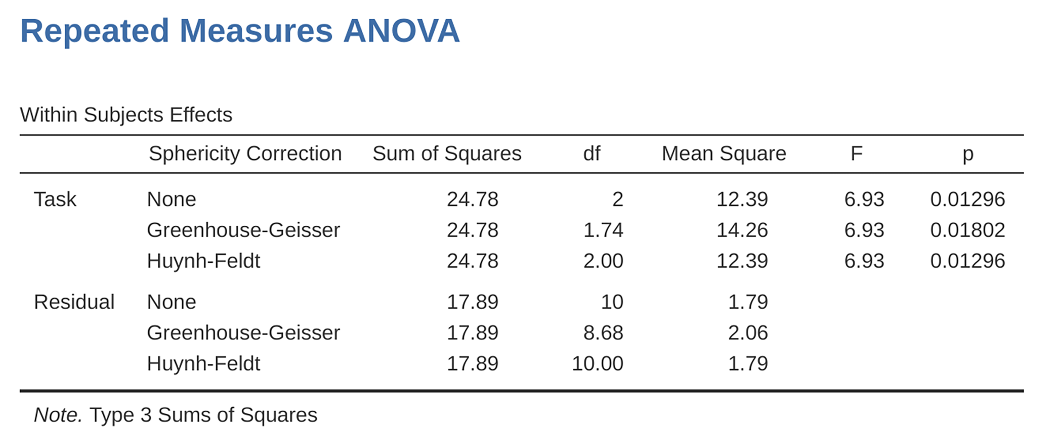
Fig. 162 Enveis ANOVA for gjentatte målinger: Test av effekter innenfor deltakere (within subjects)
In our analysis, we saw that the significance of Mauchly’s Test of Sphericity
was p = 0.720 (i.e., p > 0.05). So, this means we can assume that the
requirement of sphericity has been met so no correction to the F-value is
needed. Therefore, we can use the None Sphericity Correction output values
for the repeated measure Task: F = 6.93, df1 = 2, df2 = 10,
p = 0.013, and we can conclude that the number of tests successfully
completed on each language task did vary significantly depending on whether
the task was speech, comprehension or syntax based (F(2,10) = 6.93,
p = 0.013).
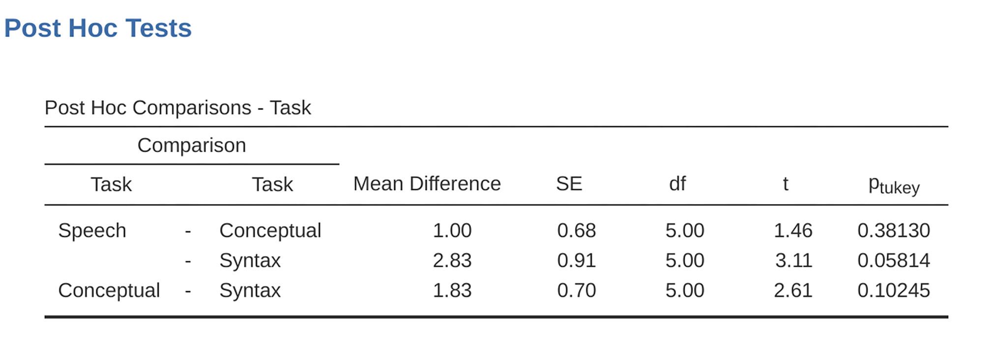
Fig. 163 Post-hoc-tester i ANOVA for gjentatte målinger i jamovi
Post-hoc tests can also be specified in jamovi for repeated measures ANOVA in
the same way as for an independent ANOVA. The results are shown in
Fig. 163. These indicate that there is a significant difference
between Speech and Syntax, but not between other levels.
Descriptive statistics (marginal means) can be reviewed to help interpret the
results, produced in the jamovi output as in Fig. 164. Comparison of
the mean number of trials successfully completed by participants shows that
Broca’s Aphasics perform reasonably well on speech production (mean = 7.17) and
language comprehension (mean = 6.17) tasks. However, their performance was
considerably worse on the syntax task (mean = 4.33), with a significant
difference in post-hoc tests between Speech and Syntax task
performance.
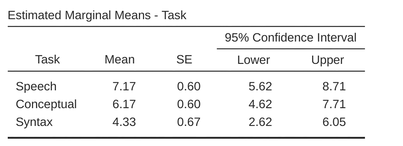
Fig. 164 Enveis ANOVA for gjentatte målinger: Deskriptivstatistikk