Autore della sezione: Danielle J. Navarro and Sebastian Jentschke

Reshaping data sets

One of the most annoying tasks that you need to undertake on a regular basis is that of reshaping a data set. Framed in the most general way, reshaping the data means taking the data in whatever format it is given to you, and converting it to the format you need it.

Long form and wide form data: The most common format in which you might obtain data is as a “case by variable” layout, commonly known as the wide format of the data. To get a sense of what I am talking about, consider an experiment in which we are interested in the different effects that alcohol and and caffeine have on people’s working memory capacity (WMC) and reaction times (RT). We recruit 10 participants, and measure their WMC and RT under three different conditions: a no drug condition, in which they are not under the influence of either caffeine or alcohol, a caffeine condition, in which they are under the inflence of caffeine, and an alcohol condition, in which… well, you can probably guess. Ideally, I suppose, there would be a fourth condition in which both drugs are administered, but for the sake of simplicity let us ignore that. The drugs data set in Fig. 49 gives you a sense of what kind of data you might observe in an experiment like this.

Fig. 49 Data table of the drugs data set in wide format

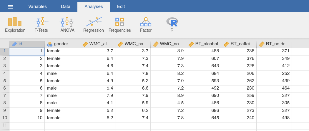
This is a data set in “wide format”, in which each participant corresponds to a single row. We have two variables that are characteristics of the subject (i.e., their id number and their gender) and six variables that refer to one of the two measured variables (WMC or RT) in one of the three testing conditions (alcohol, caffeine or no drug). Because all of the testing conditions (i.e., the three drug types) are applied to all participants, drug type is an example of a within-subject factor.

Reshaping the data set from wide to long format

The “wide format” of this data set is useful for some situations: it is often very useful to have each row correspond to a single subject. However, it is not the only way in which you might want to organise this data. For instance, you might want to have a separate row for each “testing occasion”. That is, “participant 1 under the influence of alcohol” would be one row, and “participant 1 under the influence of caffeine” would be another row. This way of organising the data is generally referred to as the long format of the data.

It is not too difficult to switch between wide and long format. We use the drugs data set, in connection with the function Wide to Long from jTransform. In the analysis panel (Fig. 50), we will find three different options regarding how the transformation can be carried out, shown as different tabs under the heading Mode at the top of the analysis panel. Quite often, the names of the original variables to be transformed (in our case, e.g., RT_caffeine or WMC_alcohol) have a separator in the variable name (in our case the _ between WMC or RT and the conditions caffeine, etc.), and follow a very clear scheme. Whenever you have a variable with a name like WMC_caffeine you know that the variable being measured is “WMC”, and that the specific condition in which it is being measured is the “caffeine” condition. Similarly, you know that RT_no.drug refers to the “RT“ variable measured in the “no drug” condition. The measured variable comes first (e.g., WMC), followed by a separator character (in this case the separator is an underscore, _), and then the name of the condition in which it is being measured (e.g., caffeine). There are two different prefixes (i.e, the strings before the separator, WMC, RT) which means that there are two separate variables being measured. There are three different suffixes (i.e., the strings after the separtator, caffeine, alcohol, no.drug) meaning that there are three different levels of the within-subject factor. Finally, notice that the separator string (i.e., _) does not appear anywhere in two of the variables (id, gender), indicating that these are between-subject variables, namely variables that do not vary within participant (e.g., a person’s gender is the same regardless of whether they’re under the influence of alcohol, caffeine etc).

Since we have this naming scheme for the variables (using _ as separator), we choose Separated as Mode. Conveniently, the _ is already present in the input box Separator. If we had another separotor (e.g., . is quite common), we would have to adjust the entry in that input box. Afterwards, we assign the within-subject factors (i.e., all WMC_… and RT_… variables) to Variables To Be Transformed, the between-subjects factor (i.e., gender) to Variables NOT To Be Transformed, and the id variable to Variables To Identify the Same Unit (see Fig. 50). To have such an ID variable is not mandatory though. If no such variable is given, the function automatically generates such an ID variable (named ID and appearing as the first column of the data set). Remember that in long format, we have several entries for each participant, therefore such ID variable is required. When checking the Data Preview, we realize that RT and WMC appear as cond1 in the preview, whereas we would like to keep them as separate variables. We can achieve this by entering 1 into the input box Exclude Level (if we take the original variable names, e.g., WMC_alcohol and split it using the separator _, then WMC and RT are the first part / level of the split variable). Now, the Data Preview looks like we intended. In addition, Repeated Measures Levels provides further information about how the variables are to be transformed. After checking both of them, we know whether the transformation will lead to the result we intended, and, if so, we can use the Create-button to open the data set transformed into long format in a new jamovi window.

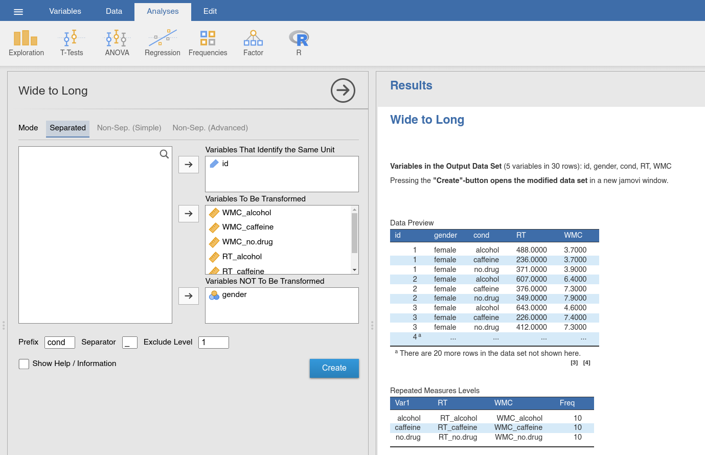
Fig. 50 Option and results panels for the Wide to Long-function from jTransform using the drugs data set

In Fig. 51, the data set that we have transformed to long format is shown. It has 30 rows: Each of the ten participants appears in three separate rows, one corresponding to each of the three conditions. And instead of having a variable like WMC_caffeine that indicates that we were measuring “WMC” in the “caffeine” condition, this information is now recorded in two separate variables, one called cond1 (that you easily could change into a more descriptive name like drug) and another called WMC. Obviously, the long and wide format of the data contain the same information, but they represent quite different ways of organising that information. Sometimes you will find that you would like to analyse data in wide form, and sometimes you find that you need long format. So it is really useful to know how to switch between the two.

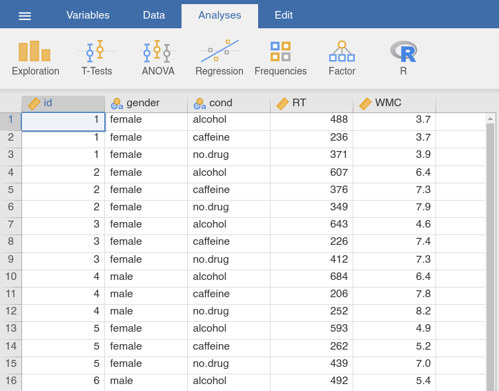
Fig. 51 Data table of the drugs_long data set in long format

Following a similar approach, we could use the Wide to Long function for situations with several experimental conditions. Consider the following, fairly simple psychological experiment. I am interested in the effects of practice on some simple decision making problem, using two distinct outcome variables. Firstly, I care about people’s accuracy, measured by the proportion of decisions that people make correctly, denoted PC. Secondly, I care about people’s speed, measured by the mean response time taken to make those decisions, denoted MRT. That is standard in psychological experiments: the speed-accuracy trade-off is pretty ubiquitous, so we generally need to care about both variables. To look at the effects of practice over the long term, I test each participant on two days, day1 and day2, where for the sake of argument I will assume that day1 and day2 are about a week apart. To look at the effects of practice over the short term, the testing during each day is broken into two “blocks”, block1 and block2, which are about 20 minutes apart. This is not the world’s most complicated experiment, but it is still a fair bit more complicated than the last one. This time around we have two within-subject factors (i.e., day and block) and we have two measured variables for each condition (i.e., PC and MRT).

Fig. 52 Data table of the choice data set in wide format

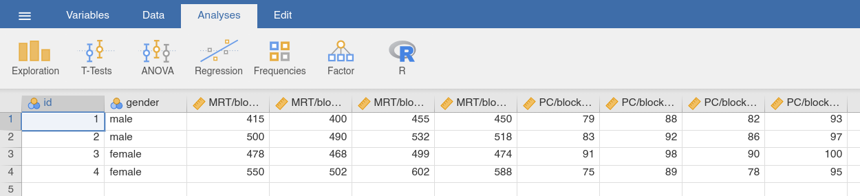
The choice data set in Fig. 52 shows what the wide form of this kind of data might look like. Notice that this time around we have variable names of the form MRT/block1/day2. As before, the first part of the name refers to the measured variable (response time), but there are now two suffixes, one indicating that the testing took place in block 1, and the other indicating that it took place on day 2. To complicate matters, it uses / as the separator character rather than _. Even so, reshaping this data set is pretty easy.

Once again, we use the Wide to Long-function, assign / to the input box Separator, the within-subject factors (i.e., all MRT_… and PC_… variables) to Variables To Be Transformed, the between-subjects factor (i.e., gender) to Variables NOT To Be Transformed, the id variable to Variables To Identify the Same Unit, and put 1 into the input box Exclude Level. We briefly check that the Data Preview and the Repeated Measures Levels look like we intended, and then use the Create-button to open the data set transformed into long format in a new jamovi window.

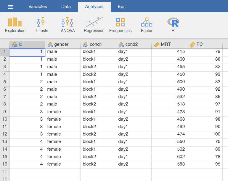
Fig. 53 Data table of the choice_long data set in long format

The resulting data set (Fig. 53) contains two between-subject variables (id and gender), two variables that define our within-subject manipulations (cond1 and cond2), and two more contain the measurements we took (MRT and PC). For clarity, it is recommended to rename cond1 into block and cond2 into day in the resulting data set.

When using the Wide to Long function, the two other modes, Non-Sep. (Simple) and Non-Sep. (Complex) provide additional flexibility for cases where the variable names do not follow a clear naming scheme. Non-Sep. (Simple) permits a set of variables (i.e., WMC_alcohol, WMC_caffeine, WMC_no.drug, RT_alcohol, RT_caffeine, RT_no.drug) to be transformed into an index variable (numbering the original set, i.e., 1 to 6) and a target variable (with var as default name). Given that we have two measurements here (WMC and RT) this is not a very useful transformation for this particular data set, but there may be other data sets where this transformation is useful.

Non-Sep. (Complex) permits several within-subject measures, and is used as shown in Fig. 54. You will have to define each measurement or target variable by replacing long_y with the name of that variable, i.e., WMC and RT to each of which you then assign all original variables of this category in the variable box underneath (e.g., are all WMC_… assigned to WMC). Afterwards, you need to define Name and N Levels for each index variable Index Variable (Can Be Nested) (each class of conditions would be represented by one index variable), for the current data set we may choose condition as name, and 3 as the number of levels. For the choice data set, the target variables would be MRT and PC, and we would have to index variables, block and day with 2 levels each.

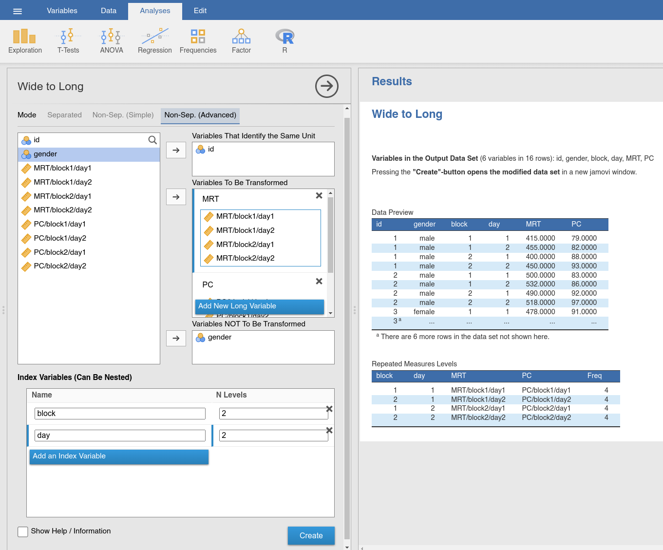
Fig. 54 Option and results panels for the Wide to Long-function from jTransform using the choice data set and the mode Non-Sep (Advanced)

Reshaping the data set from long to wide format

To convert data from long form to wide format, we can use the Long to Wide function from the jTransform module. We can use the data set that we just transformed (Fig. 51; the same data set is available as drugs_long). Recall from earlier that this data set in long format contains variables named id, gender, drug (or cond, if we did not change the name), WMC and RT. In order to convert from long form to wide form you will need the following setup in your options panel (Fig. 55). Here, you need to indicate which of these variables are measured separately for each condition (i.e., WMC and RT), these variables are assigned to Variables To Be Transformed; and which variable is the within-subject factor that specifies the condition (i.e., drug or cond), this variable is assigned to Variables That Differentiate Within a Unit. It was mentioned earlier, that in data sets with long format it is mandatory to have an ID variable (here id) which is assigned to Variables That Identify the Same Unit. Finally, if we have a between-subjects factor (in our case gender), we assign this variable to Variables Not To Be Transformed. Again, we check the Data Preview and the Repeated Measures Levels, and use the Create-button once these two outputs indicate that the transformation gives us the intended result.

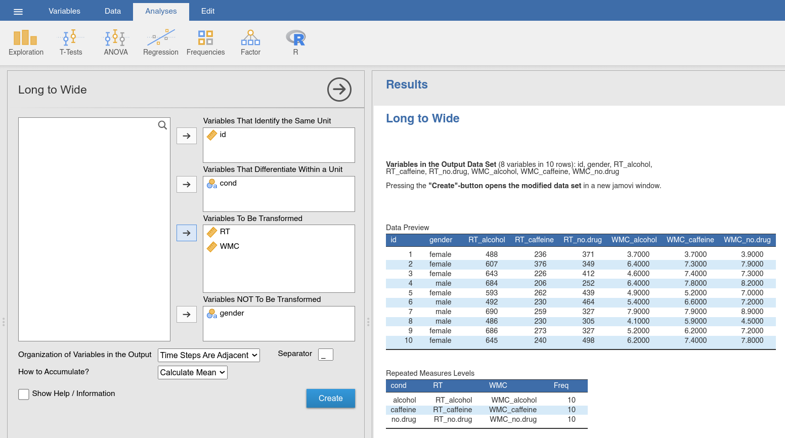
Fig. 55 Option and results panels for the Long to Wide-function from jTransform using the drugs_long data set

In the same way, we could convert back the transformation of the choice data set into long format. We use the Long to Wide function, assigning the measures (i.e., PC and MRT) to Variables To Be Transformed, the within-subject factor that specifies the condition (i.e., cond1 and cond2 or day and block if we changed the names) to Variables That Differentiate Within a Unit, the ID variable (id) to Variables That Identify the Same Unit, and the between-subjects factor (gender) to Variables Not To Be Transformed. Again, we check the Data Preview and the Repeated Measures Levels, and use the Create-button once these two outputs indicate that the transformation gives us the intended result. This produces a data set in wide format containing the same variables as the original choice data set.

Finally, the Long to Wide function implements an option to accumulate data over conditions. Let us assume that we after all decide that we are only interested in the long-term effects (day1 vs. day2). We would then use the Long to Wide function (Fig. 56), assign the measures (i.e., PC and MRT) to Variables To Be Transformed, the within-subject factor that specifies the condition we would like to keep (i.e., cond2 or day) to Variables That Differentiate Within a Unit, the ID variable (id) to Variables That Identify the Same Unit, and the between-subjects factor (gender) to Variables Not To Be Transformed. The function would then calculate the mean (or take the first value, depending on what setting we choose for How to Accumulate) over the occurences of cond1 or block. You can get an impression of the difference when you compare the Data Preview while adding and removing the cond1 or block variable to Variables To Be Transformed.

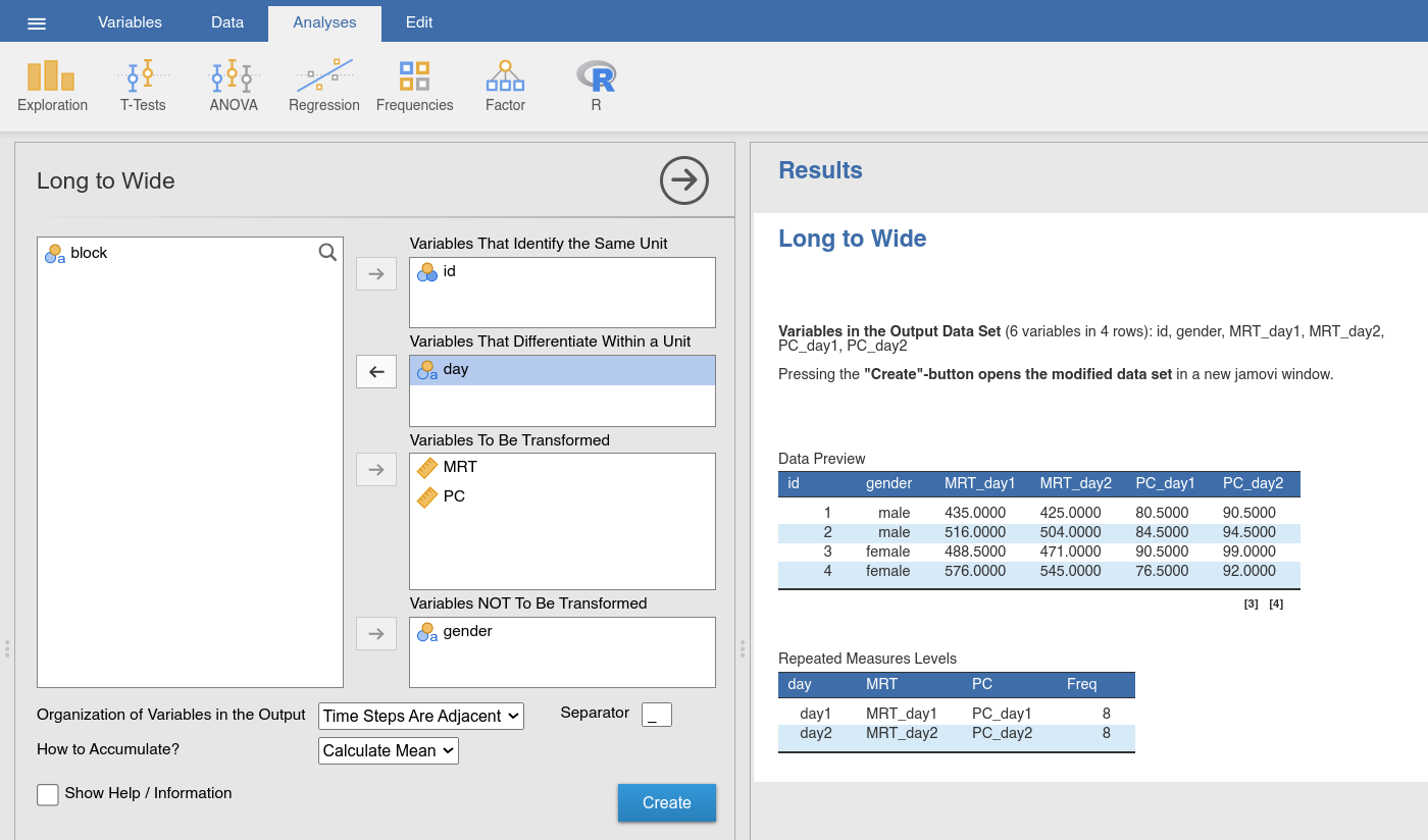
Fig. 56 Option and results panels for the Long to Wide-function from jTransform using the choice_long data set and accumulating over the condition block

The advantage to the functions described in the previous section is that they solve (commonly encountered) problems with a minimum of fuss. The disadvantage is that these function are relatively limited in scope.

For more advanced operations, one may have to use R-code. There are two approaches for doing that. The first, and easier, approach is to use the Rj editor (one of the numerous jamovi modules). There you can carry out manipulations on the data set you have currently opened in your jamovi session (you can access it as data in the Rj editor) and afterwards you can open the manipulated data set in a new jamovi session using the openNew-function. The second approach is to open your data set in an R-session, using the function read_omv from the R-package jmvReadWrite (cf. Syntax mode). Alternatively, for creating a new data set, you would read information from, e.g., log files, using the R-function read.csv, extract the information you need from those files into one data frame which you then write into a format that can be opened in jamovi (using, e.g., saveRDS from base R or write_omv from jmvReadWrite).