Autor des Abschnitts: Danielle J. Navarro and David R. Foxcroft
Der t-Test für gepaarte Stichproben
Regardless of whether we are talking about the Student test or the Welch test, an independent samples t-test is intended to be used in a situation where you have two samples that are, well, independent of one another. This situation arises naturally when participants are assigned randomly to one of two experimental conditions, but it provides a very poor approximation to other sorts of research designs. In particular, a repeated measures design, in which each participant is measured (with respect to the same outcome variable) in both experimental conditions, is not suited for analysis using independent samples t-tests. For example, we might be interested in whether listening to music reduces people’s working memory capacity. To that end, we could measure each person’s working memory capacity in two conditions: with music, and without music. In an experimental design such as this one,[1] each participant appears in both groups. This requires us to approach the problem in a different way, by using the paired samples t-test.
Die Daten
The data set that we will use this time comes from Dr Chico’s class.[2]
In her class students take two major tests, one early in the semester
and one later in the semester. To hear her tell it, she runs a very hard
class, one that most students find very challenging. But she argues that
by setting hard assessments students are encouraged to work harder. Her
theory is that the first test is a bit of a “wake up call” for students.
When they realise how hard her class really is, they will work harder for
the second test and get a better mark. Is she right? To test this, let us
import the chico data set into jamovi. This time jamovi does a good
job during the import of attributing measurement levels correctly. The
chico data set contains three variables: an id variable that
identifies each student in the class, the grade_test1 variable that
records the student grade for the first test, and the grade_test2
variable that has the grades for the second test.
If we look at the jamovi spreadsheet it does seem like the class is a hard one (most grades are between 50% and 60%), but it does look like there is an improvement from the first test to the second one.
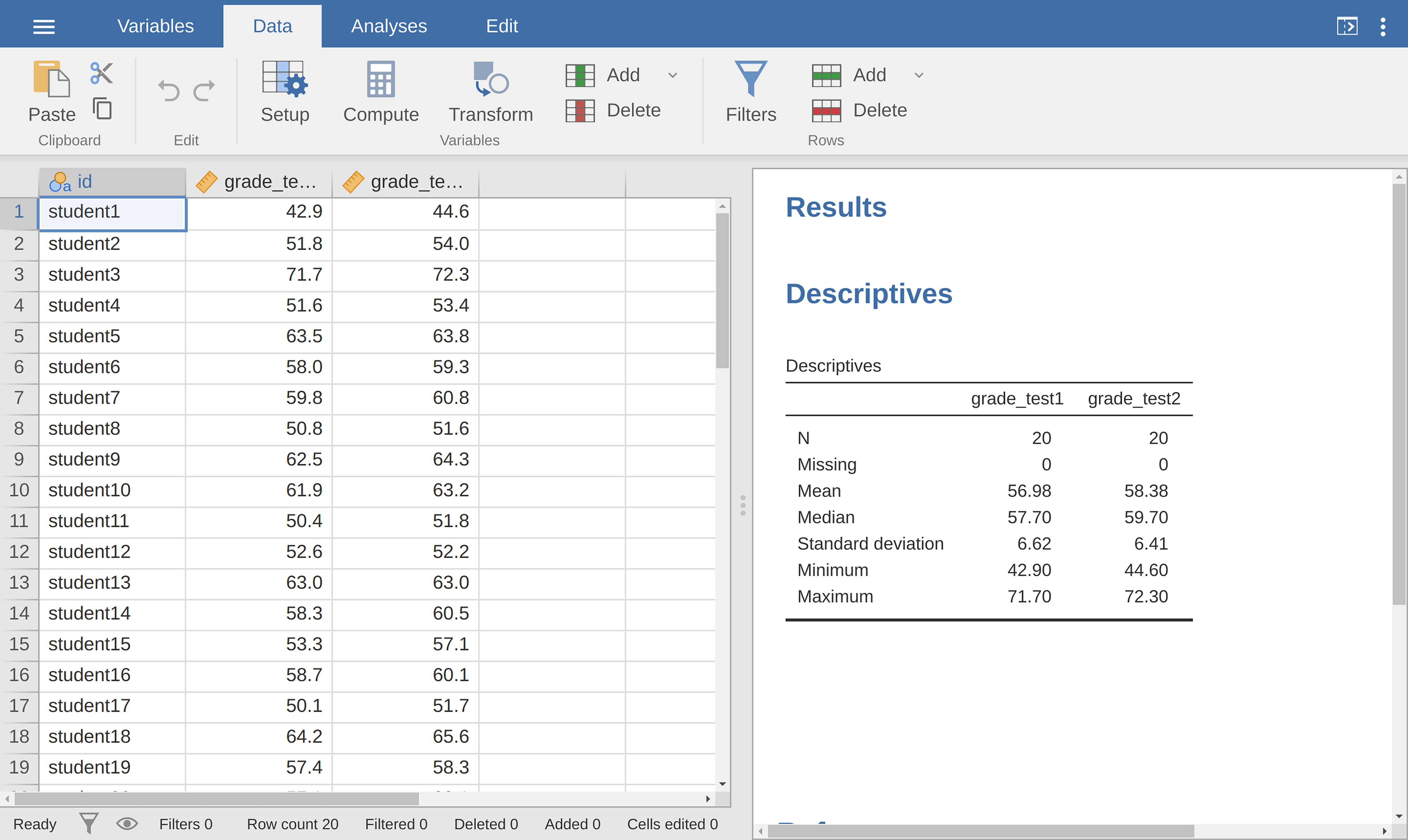
Abb. 108 Deskriptivstatistik für die Variablen mit den zwei Examensnoten aus dem chico-Datensatz
If we take a quick look at the descriptive statistics, in Abb. 108, we see that this impression seems to be supported. Across all 20 students the mean grade for the first test is 57%, but this rises to 58% for the second test. Although, given that the standard deviations are 6.6% and 6.4% respectively, it is starting to feel like maybe the improvement is just illusory; maybe just random variation. This impression is reinforced when you see the means and confidence intervals plotted in Abb. 109 (left panel). If we were to rely on this plot alone, looking at how wide those confidence intervals are, we would be tempted to think that the apparent improvement in student performance is pure chance.

|

|

Abb. 109 Mean grade for test 1 and test 2, with associated 95% confidence intervals (left panel). Scatterplot showing the individual grades for test 1 and test 2 (right panel).
Nevertheless, this impression is wrong. To see why, take a look at the
scatterplot of the grades for test 1 against the grades for test 2, shown in
Abb. 109 (right panel). In this plot each dot corresponds to the
two grades for a given student. If their grade for test 1 (x co-ordinate)
equals their grade for test 2 (y co-ordinate), then the dot falls on the
line. Points falling above the line are the students that performed better on
the second test. Critically, almost all of the data points fall above the
diagonal line: almost all of the students do seem to have improved their
grade, if only by a small amount. This suggests that we should be looking at
the improvement made by each student from one test to the next and treating
that as our raw data. To do this, we will need to create a new variable for the
improvement that each student makes, and add it to the chico data set.
The easiest way to do this is to compute a new variable, with the expression
grade_test2 - grade_test1.
Once we have computed this new improvement variable we can draw a histogram
showing the distribution of these improvement scores, shown in
Abb. 110. When we look at the histogram, it is very clear that there
is a real improvement here. The vast majority of the students scored higher
on test 2 than on test 1, reflected in the fact that almost the entire histogram
is above zero.

Abb. 110 Histogram from jamovi showing the improvement made by each student in Dr Chico’s class. Notice that almost the entire distribution is above zero – the vast majority of students did improve their performance from the first test to the second one.
Was macht der t-Test für gepaarte Stichproben?
In light of the previous exploration, let us think about how to construct an
appropriate t-test. One possibility would be to try to run an independent
samples t-test using grade_test1 and grade_test2 as the variables of
interest. However, this is clearly the wrong thing to do as the independent
samples t-test assumes that there is no particular relationship between the
two samples. Yet clearly that is not true in this case because of the repeated
measures structure in the data. To use the language that I introduced in the
last section, if we were to try to do an independent samples t-test, we would
be conflating the within subject differences (which is what we are
interested in testing) with the between subject variability (which we are
not).
Die Lösung des Problems ist hoffentlich offensichtlich, da wir die ganze harte Arbeit bereits im vorherigen Abschnitt erledigt haben. Anstatt einen t-Test für unabhängige Stichproben mit grade_test1 und grade_test2 durchzuführen, führen wir einen t-Test für eine Stichprobe mit der Variable für die Differenz innerhalb des Subjekts, improvement, durch. Um dies zu formalisieren: Wenn X:sub`i1` die Punktzahl ist, die der i-te Teilnehmer bei der ersten Variable erreicht hat, und X:sub`i2` die Punktzahl ist, die dieselbe Person bei der zweiten Variable erreicht hat, dann ist die Differenzpunktzahl:
Notice that the difference scores is variable 1 minus variable 2 and not the other way around, so if we want improvement to correspond to a positive valued difference, we actually want “test 2” to be our “variable 1”. Equally, we would say that µD = µ1 - µ2 is the population mean for this difference variable. So, to convert this to a hypothesis test, our null hypothesis is that this mean difference is zero and the alternative hypothesis is that it is not:
This is assuming we are talking about a two-sided test here. This is more or less identical to the way we described the hypotheses for the one-sample t-test. The only difference is that the specific value that the null hypothesis predicts is 0. And so our t-statistic is defined in more or less the same way too. If we let D̄ denote the mean of the difference scores, then:
which is:
where \(\hat\sigma_D\) is the standard deviation of the difference scores. Since this is just an ordinary, one-sample t-test, with nothing special about it, the degrees of freedom are still N - 1. And that is it. The paired samples t-test really is not a new test at all. It is a one-sample t-test, but applied to the difference between two variables. It is actually very simple. The only reason it merits a discussion as long as the one we have just gone through is that you need to be able to recognise when a paired samples test is appropriate, and to understand why it is better than an independent samples t-test.
Durchführen des Tests in jamovi
How do you do a paired samples t-test in jamovi? One possibility is to follow
the process I outlined above. That is, create a difference variable and then
run a one sample t-test on that. Since we have already created a variable
called improvement, let us do that and see what we get (see
Abb. 111).
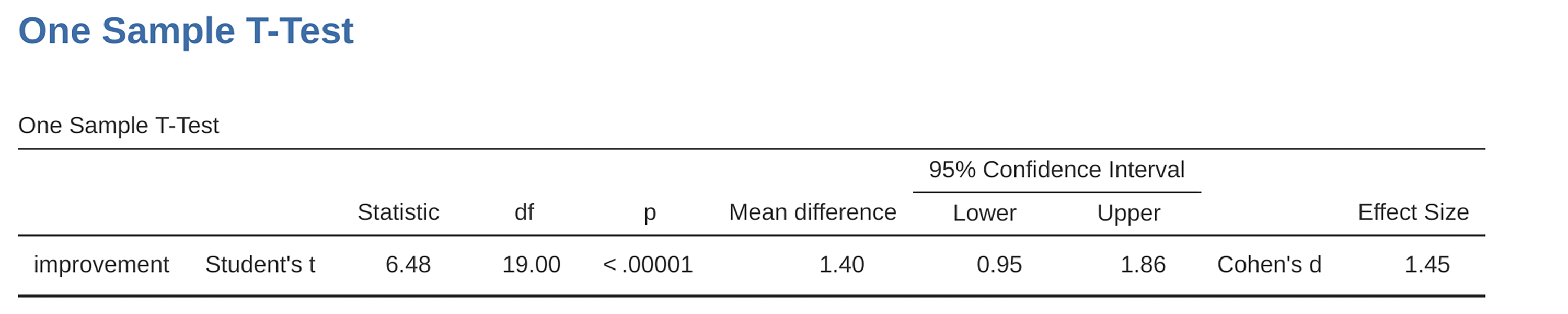
Abb. 111 Die Ergebnisse zeigen einen t-Test mit paarweisen Differenzwerten
The output shown in Abb. 111 is (obviously) formatted exactly the
same was as it was the last time we used the One Sample T-Test analysis
(section Der t-Test bei einer Stichprobe), and it confirms our intuition. There is an
average improvement of 1.4% from test 1 to test 2, and this is significantly
different from 0 (t(19) = 6.48, p < 0.001).
However, suppose you are lazy and you do not want to go to all the effort of
creating a new variable. Or perhaps you just want to keep the difference
between one-sample and paired-samples tests clear in your head. If so, you can
use the jamovi Paired Samples T-Test analysis, getting the results shown in
Abb. 112.
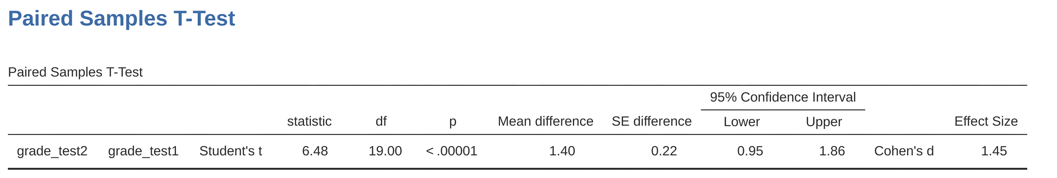
Abb. 112 Results showing a paired sample t-test. Compare it with Abb. 111.
Die Zahlen sind identisch mit denen des Einstichprobentests, was sie natürlich auch sein müssen, da der t-Test für gepaarte Stichproben unter der Haube ein t-Test für eine Stichprobe ist.