Autor des Abschnitts: Danielle J. Navarro and David R. Foxcroft

Der χ²-Unabhängigkeitstest

GUARDBOT 1:	Halt!
GUARDBOT 2:	Bist du ein Roboter oder ein Mensch?
LEELA:	Roboter… sind wir.
FRY:	Äh, ja! Nur zwei Roboter, die sich die Köpfe einschlagen! Was?
GUARDBOT 1:	Führen Sie den Test durch.
GUARDBOT 2:	Welche der folgenden Optionen würden Sie am meisten bevorzugen? A: Einen Hundewelpen, B: Eine hübsche Blume von Ihrer Liebsten oder C: Eine große, richtig formatierte Datei?
GUARDBOT 1:	Wählen Sie!

—Futurama, „Angst vor einem Bot-Planeten“

The other day I was watching an animated documentary examining the quaint customs of the natives of the planet Chapek 9. Apparently, in order to gain access to their capital city a visitor must prove that they are a robot, not a human. In order to determine whether or not a visitor is human, the natives ask whether the visitor prefers puppies, flowers, or large, properly formatted data files. “Pretty clever,” I thought to myself “but what if humans and robots have the same preferences? That probably would not be a very good test then, would it?” As it happens, I got my hands on the testing data that the civil authorities of Chapek 9 used to check this. It turns out that what they did was very simple. They found a bunch of robots and a bunch of humans and asked them what they preferred. I saved their data in the chapek9 data set, which we can now load into jamovi. As well as the ID variable that identifies individual people, there are two nominal text variables , species and choice. In total there are 180 entries in the data set, one for each person (counting both robots and humans as “people”) who was asked to make a choice. Specifically, there are 93 humans and 87 robots, and overwhelmingly the preferred choice is the data file. You can check this yourself by asking jamovi for Frequency Tables, under the Exploration → Descriptives button. However, this summary does not address the question we are interested in. To do that, we need a more detailed description of the data. What we want to do is look at the choices broken down by species. That is, we need to cross-tabulate the data (see Erstellen von Häufigkeitstabellen und Kreuztabellen aus Ihren Daten). In jamovi we do this using the Frequencies → Contingency Tables → Independent Samples analysis, and we should get a table something like this:

	Roboter	Menschen	Insgesamt
Welpe	13	15	28
Blume	30	13	43
Daten	44	65	109
Insgesamt	87	93	180

From this, it is quite clear that the vast majority of the humans chose the data file, whereas the robots tended to be a lot more even in their preferences. Leaving aside the question of why the humans might be more likely to choose the data file for the moment (which does seem quite odd, admittedly), our first order of business is to determine if the discrepancy between human choices and robot choices in the data set is statistically significant.

Aufbau unseres Hypothesentests

Wie können wir diese Daten analysieren? Da meine Forschungs-Hypothese lautet, dass „Menschen und Roboter die Frage auf unterschiedliche Weise beantworten“, wie kann ich einen Test der Nullhypothese konstruieren, dass „Menschen und Roboter die Frage auf dieselbe Weise beantworten“? Wie zuvor beginnen wir mit der Festlegung einer Notation zur Beschreibung der Daten:

	Roboter	Menschen	Insgesamt
Welpe	O11	O12	R1
Blume	O21	O22	R2
Daten	O31	O32	R3
Insgesamt	C1	C2	N

In this notation we say that O_ij is a count (observed frequency) of the number of respondents that are of species j (robots or human) who gave answer i (puppy, flower or data) when asked to make a choice. The total number of observations is written N, as usual. Finally, I have used R_i to denote the row totals (e.g., R₂ is the total number of creatures who chose the flower), and C_j to denote the column totals (e.g., C₁ is the total number of robots).[1]

So now let us think about what the null hypothesis says. If robots and humans are responding in the same way to the question, it means that the probability that “a robot says puppy” is the same as the probability that “a human says puppy”, and so on for the other two possibilities. So, if we use P_ij to denote “the probability that a member of species j gives response i” then our null hypothesis is that:

H0:	Alle folgenden Aussagen sind wahr:
	P11 = P12 (gleiche Wahrscheinlichkeit, „Welpe“ zu sagen),
	P21 = P22 (gleiche Wahrscheinlichkeit, „Blume“ zu sagen), und
	P31 = P32 (gleiche Wahrscheinlichkeit, „Daten“ zu sagen).

And actually, since the null hypothesis is claiming that the true choice probabilities do not depend on the species of the person making the choice, we can let P_i refer to this probability, e.g., P₁ is the true probability of choosing the puppy.

Next, in much the same way that we did with the goodness-of-fit test, what we need to do is calculate the expected frequencies. That is, for each of the observed counts O_ij, we need to figure out what the null hypothesis would tell us to expect. Let us denote this expected frequency by E_ij. This time, it is a little bit trickier. If there are a total of C_j people that belong to species j, and the true probability of anyone (regardless of species) choosing option i is P_i, then the expected frequency is just:

E_ij = C_j · P_i

Now, this is all very well and good, but we have a problem. Unlike the situation we had with the goodness-of-fit test, the null hypothesis does not actually specify a particular value for P_i. It is something we have to estimate from the data! Fortunately, this is pretty easy to do. If 28 out of 180 people selected the flowers, then a natural estimate for the probability of choosing flowers is 28 / 180, which is approximately 0.16. If we phrase this in mathematical terms, what we are saying is that our estimate for the probability of choosing option i is just the row total divided by the total sample size:

\[\hat{P}_i = \frac{R_i}{N}\]

Daher ergibt sich die erwartete Häufigkeit als das Produkt (d. h. die Multiplikation) der Zeilensumme und der Spaltensumme, geteilt durch die Gesamtzahl der Beobachtungen:[2]

Ê_ij = (R_i · C_j) / N

Now that we have figured out how to calculate the expected frequencies, it is straightforward to define a test statistic, following the exact same strategy that we used in the goodness-of-fit test. In fact, it is pretty much the same statistic.

For a contingency table with r rows and c columns, the equation that defines our χ² statistic is:

\[\chi ^ 2 = \sum_{i = 1} ^ r \sum_{j = 1} ^ c \frac{({E}_{ij} - O_{ij}) ^ 2}{{E}_{ij}}\]

The only difference is that I have to include two summation signs (i.e., Σ) to indicate that we are summing over both rows and columns.

Wie zuvor deuten große Werte von χ² darauf hin, dass die Nullhypothese die Daten schlecht beschreibt, während kleine Werte von χ² darauf hindeuten, dass sie die Daten gut wiedergibt. Daher werden wir, wie beim letzten Mal, die Nullhypothese verwerfen, wenn χ² zu groß ist.

Not surprisingly, this statistic is χ² distributed. All we need to do is figure out how many degrees of freedom are involved, which actually is not too hard. As I mentioned before, you can (usually) think of the degrees of freedom as being equal to the number of data points that you are analysing, minus the number of constraints. A contingency table with r rows and c columns contains a total of r · c observed frequencies, so that is the total number of observations. What about the constraints? Here, it is slightly trickier. The answer is always the same:

df = (r - 1)(c - 1)

However, the explanation for why the degrees of freedom takes this value is different depending on the experimental design. For the sake of argument, let us suppose that we had honestly intended to survey exactly 87 robots and 93 humans (column totals fixed by the experimenter), but left the row totals free to vary (row totals are random variables). Let us think about the constraints that apply here. Well, since we deliberately fixed the column totals by Act of Experimenter, we have c constraints right there. But, there is actually more to it than that. Remember how our null hypothesis had some free parameters (i.e., we had to estimate the P_i values)? Those matter too. I will not explain why in this book, but every free parameter in the null hypothesis is rather like an additional constraint. So, how many of those are there? Well, since these probabilities have to sum to 1, there is only r - 1 of these. So our total degrees of freedom is:

\[\begin{split}\begin{array}{rcl} $df$ & = & \mbox{(number of observations)} - \mbox{(number of constraints)} \\ & = & (rc) - (c + (r - 1)) \\ & = & rc - c - r + 1 \\ & = & (r - 1)(c - 1) \end{array}\end{split}\]

Alternatively, suppose that the only thing that the experimenter fixed was the total sample size N. That is, we quizzed the first 180 people that we saw and it just turned out that 87 were robots and 93 were humans. This time around our reasoning would be slightly different, but would still lead us to the same answer. Our null hypothesis still has r - 1 free parameters corresponding to the choice probabilities, but it now also has c - 1 free parameters corresponding to the species probabilities, because we would also have to estimate the probability that a randomly sampled person turns out to be a robot.[3] Finally, since we did actually fix the total number of observations N, that is one more constraint. So, now we have rc observations, and (c - 1) + (r - 1) + 1 constraints. What does that give?

\[\begin{split}\begin{array}{rcl} $df$ & = & \mbox{(number of observations)} - \mbox{(number of constraints)} \\ & = & rc - ( (c - 1) + (r - 1) + 1) \\ & = & rc - c - r + 1 \\ & = & (r - 1)(c - 1) \end{array}\end{split}\]

Erstaunlich.

Durchführen des Tests in jamovi

Okay, now that we know how the test works let us have a look at how it is done in jamovi. As tempting as it is to lead you through the tedious calculations so that you are forced to learn it the long way, I figure there is no point. I already showed you how to do it the long way for the goodness-of-fit test in the last section, and since the test of independence is not conceptually any different, you will not learn anything new by doing it the long way. So instead I will go straight to showing you the easy way. After you have run the test in jamovi (Frequencies → Contingency Tables → Independent Samples), all you have to do is look underneath the contingency table in the jamovi results window and there is the χ² statistic for you. This shows a χ² statistic value of 10.72, with df = 2 and a p-value = 0.005.

That was easy, was not it! You can also ask jamovi to show you the expected counts – just click on the check box for Expected Counts in the Cells options and the expected counts will appear in the contingency table. And whilst you are doing that, an effect size measure would be helpful. We will choose Phi and Cramer’s V, and you can specify this from a check box in the Statistics options, and it gives a value for Cramer’s V of 0.24 (see Abb. 93). We will talk about this some more in just a moment.

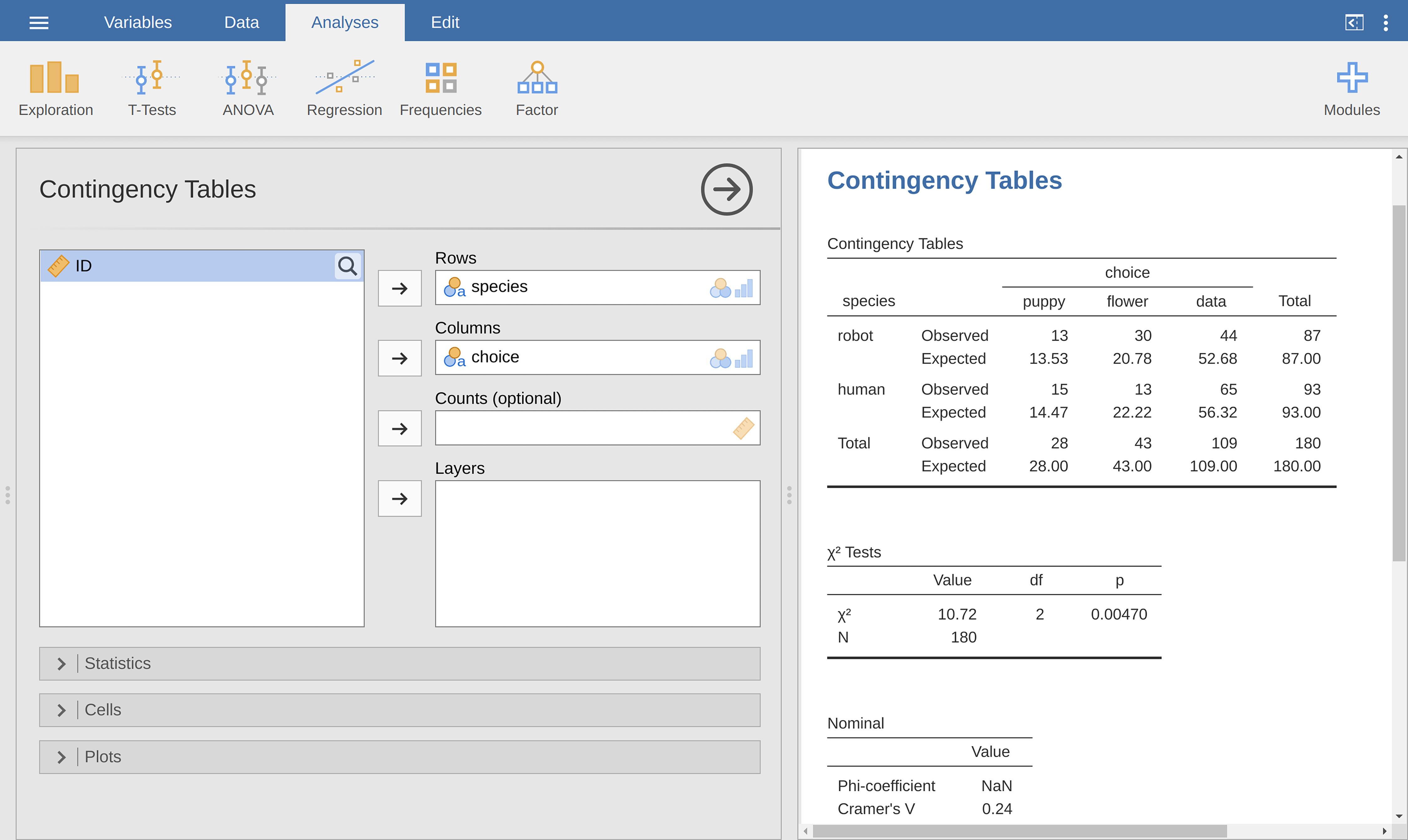
Abb. 93 Independent samples χ² test in jamovi using the chapek9 data set

Diese Ausgabe gibt uns genügend Informationen, um das Ergebnis zu berichten:

Pearson’s χ² ergab einen signifikanten Zusammenhang zwischen Spezies und Wahl (χ²(2) = 10,7, p < 0,01). Die Roboter scheinen eher zu sagen, dass sie Blumen bevorzugen, die Menschen dagegen eher, dass sie Daten bevorzugen.

Notice that, once again, I provided a little bit of interpretation to help the human reader understand what is going on with the data. Later on in my discussion section I should provide a bit more context. To illustrate the difference, here is what I probably would say later on:

Die Tatsache, dass Menschen offenbar eine stärkere Vorliebe für Daten-Dateien haben als Roboter, ist etwas kontraintuitiv. Im Kontext betrachtet, ergibt dies jedoch einen gewissen Sinn, da die Zivilbehörde auf Chapek 9 leider dazu neigt, Menschen, die identifiziert werden konnten, zu töten und zu sezieren. Daher ist es sehr wahrscheinlich, dass die menschlichen Teilnehmer nicht ehrlich auf die Frage geantwortet haben, um potenziell unerwünschte Konsequenzen zu vermeiden. Dies sollte als erhebliche methodische Schwäche betrachtet werden.

Dies kann als ein ziemlich extremes Beispiel für einen Reaktivitätseffekt eingestuft werden. Offensichtlich ist das Problem in diesem Fall so gravierend, dass die Studie als Instrument zum Verständnis der unterschiedlichen Präferenzen von Menschen und Robotern mehr oder weniger wertlos ist. Ich hoffe jedoch, dass dies den Unterschied zwischen einem statistisch signifikanten Ergebnis (unsere Nullhypothese wird zugunsten der Alternative verworfen) und einem Ergebnis von wissenschaftlichem Wert (die Daten sagen uns aufgrund eines großen methodischen Fehlers nichts Interessantes über unsere Forschungshypothese) verdeutlicht.

Nachtrag

I later found out the data were made up, and I had been watching cartoons instead of doing work.

---

[1]

A technical note. The way I have described the test pretends that the column totals are fixed (i.e., the researcher intended to survey 87 robots and 93 humans) and the row totals are random (i.e., it just turned out that 28 people chose the puppy). To use the terminology from my mathematical statistics textbook (Hogg et al., 2005), I should technically refer to this situation as a χ²-test of homogeneity and reserve the term χ²-test of independence for the situation where both the row and column totals are random outcomes of the experiment. In the initial drafts of this book that is exactly what I did. However, it turns out that these two tests are identical, and so I have collapsed them together.

[2]

Technically, E_ij here is an estimate, so I should probably write it Ê_ij. But since no-one else does, I will not either.

[3]

Ein Problem, über das sich viele von uns im wirklichen Leben Sorgen machen.