Tác giả mục:Danielle J. Navarro and David R. Foxcroft

Analysis of Covariance (ANCOVA)

A variation in ANOVA is when you have an additional continuous variable that you think might be related to the dependent variable. This additional variable can be added to the analysis as a covariate, in the aptly named analysis of covariance (ANCOVA).

In ANCOVA the values of the dependent variable are “adjusted” for the influence of the covariate, and then the “adjusted” score means are tested between groups in the usual way. This technique can increase the precision of an experiment, and therefore provide a more “powerful” test of the equality of group means in the dependent variable. How does ANCOVA do this? Well, although the covariate itself is typically not of any experimental interest, adjustment for the covariate can decrease the estimate of experimental error and thus, by reducing error variance, precision is increased. This means that an inappropriate failure to reject the null hypothesis (false negative or type II error) is less likely.

Despite this advantage, ANCOVA runs the risk of undoing real differences between groups , and this should be avoided. Look at Fig. 154, for example, which shows a plot of Statistics anxiety against age and shows two distinct groups – students who have either an Arts or Science background or preference. ANCOVA with age as a covariate might lead to the conclusion that statistics anxiety does not differ in the two groups. Would this conclusion be reasonable – probably not because the ages of the two groups do not overlap and analysis of variance has essentially “extrapolated into a region with no data” (Everitt, 1996).

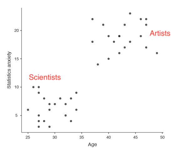
Fig. 154 Plot of Statistics anxiety against age for two distinct groups

Clearly, careful thought needs to be given to an analysis of covariance with distinct groups. This applies to both one-way and factorial designs, as ANCOVA can be used with both.

Running ANCOVA in jamovi

A health psychologist was interested in the effect of routine cycling and stress on happiness levels, with age as a covariate. Open the ancova data set in jamovi and then, to undertake an ANCOVA, select Analyses → ANOVA → ANCOVA to open the ANCOVA analysis window (Fig. 155). Highlight the dependent variable happiness and transfer it into the Dependent Variable text box. Highlight the independent variables stress and commute and transfer them into the Fixed Factors text box. Highlight the covariate age and transfer it into the Covariates text box. Then, click on Estimated Marginal Means to bring up the plots and tables options.

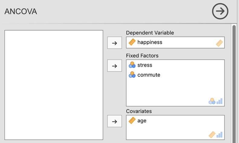
Fig. 155 Options panel showing the variable boxes to assign the Dependent Variable, Fixed Factors and the Covariates for the ANCOVA in jamovi

An ANCOVA table showing Tests of Between-Subjects Effects is produced in the jamovi results panel (Fig. 156). The F-value for the covariate age is significant at p = 0.023, suggesting that age is an important predictor of the dependent variable, happiness. When we look at the estimated marginal mean scores (Fig. 157), adjustments have been made (compared to an analysis without the covariate) because of the inclusion of the covariate age in this ANCOVA. A plot (Fig. 158) is a good way of visualising and interpreting the significant effects.

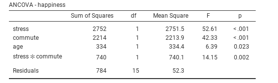
Fig. 156 jamovi ANCOVA output for happiness as a function of stress and commuting method, with age as a covariate

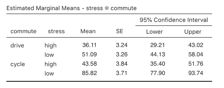
Fig. 157 Table with the Estimated Marginal means within the ANCOVA: Shown are the mean happiness level as a function of stress and commuting method (adjusted for the covariate age) with 95% confidence intervals

The F-value for the main effect stress (52.61) has an associated probability of p < 0.001. The F-value for the main effect commute (42.33) has an associated probability of p < 0.001. Since both of these are less than the probability that is typically used to decide if a statistical result is significant (p < 0.05) we can conclude that there was a significant main effect of stress (F(1,15) = 52.61, p < 0.001) and a significant main effect of commuting method (F(1,15) = 42.33, p < 0.001). A significant interaction between stress and commuting method was also found (F(1,15) = 14.15, p = 0.002).

In Fig. 158 we can see the adjusted, marginal, mean happiness scores when age is a covariate in an ANCOVA. In this analysis there is a significant interaction effect, whereby people with low stress who cycle to work are happier than people with low stress who drive and people with high stress whether they cycle or drive to work. There is also a significant main effect of stress – people with low stress are happier than those with high stress. And there is also a significant main effect of commuting behaviour – people who cycle are happier, on average, than those who drive to work.

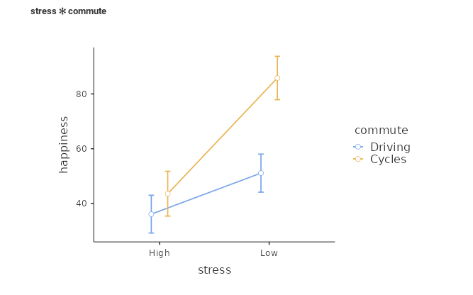
Fig. 158 Plot with the Estimated Marginal means within the ANCOVA: Shown are the mean happiness level as a function of stress and commuting method

One thing to be aware of is that, if you are thinking of including a covariate in your ANOVA, there is an additional assumption: the relationship between the covariate and the dependent variable should be similar for all levels of the independent variable. This can be checked by adding an interaction term between the covariate and each independent variable in the jamovi Model → Model terms option. If the interaction effect is not significant it can be removed. If it is significant then a different and more advanced statistical technique might be appropriate (which is beyond the scope of this book so you might want to consult a friendly statistician).