Автор раздела: Danielle J. Navarro and David R. Foxcroft

Testing non-normal data with Wilcoxon tests

Suppose your data turn out to be pretty substantially non-normal, but you still want to run something like a t-test? This situation occurs a lot in real life. For the AFL winning margins data (afl.margins from the aflsmall_margins data set), for instance, the Shapiro-Wilk test made it very clear that the normality assumption is violated. This is the situation where you want to use Wilcoxon tests.

Like the t-test, the Wilcoxon test comes in two forms, one-sample and two-sample, and they are used in more or less the exact same situations as the corresponding t-tests. Unlike the t-test, the Wilcoxon test does not assume normality, which is nice. In fact, they do not make any assumptions about what kind of distribution is involved. In statistical jargon, this makes them non-parametric tests. While avoiding the normality assumption is nice, there is a drawback: the Wilcoxon test is usually less powerful than the t-test (i.e., higher Type II error rate). I will not discuss the Wilcoxon tests in as much detail as the t-tests, but I will give you a brief overview.

Two sample Mann-Whitney U test

I will start by describing the Mann-Whitney U test, since it is actually simpler than the one sample version. Suppose we are looking at the scores of 10 people on some test. Since my imagination has now failed me completely, let us pretend it is a “test of awesomeness” and there are two groups of people, “A” and “B”. I am curious to know which group is more awesome. The data are included in the awesome data set, and there are two variables apart from the usual ID variable: scores and group .

As long as there are no ties (i.e., people with the exact same awesomeness score) then the test that we want to do is surprisingly simple. All we have to do is construct a table that compares every observation in group A against every observation in group B. Whenever the group A datum is larger, we place a check mark in the table:

		Group B
		14.5	10.4	12.4	11.7	13.0
Group A	6.4
	10.7		✓
	11.9		✓		✓
	7.3
	10.0

We then count up the number of checkmarks. This is our test statistic, U.[1] The actual sampling distribution for U is somewhat complicated, and I will skip the details. For our purposes, it is sufficient to note that the interpretation of U is qualitatively the same as the interpretation of t or z. That is, if we want a two-sided test then we reject the null hypothesis when U is very large or very small, but if we have a directional (i.e., one-sided) hypothesis then we only use one or the other.

In jamovi, if we run an Independent Samples T-Test with scores as the dependent variable. and group as the grouping variable , and then under the options for Tests check the option for Mann-Whitney U, we will get results showing that U = 3 (i.e., the same number of check marks as shown above), and a p-value = 0.05556 (Рис. 122).

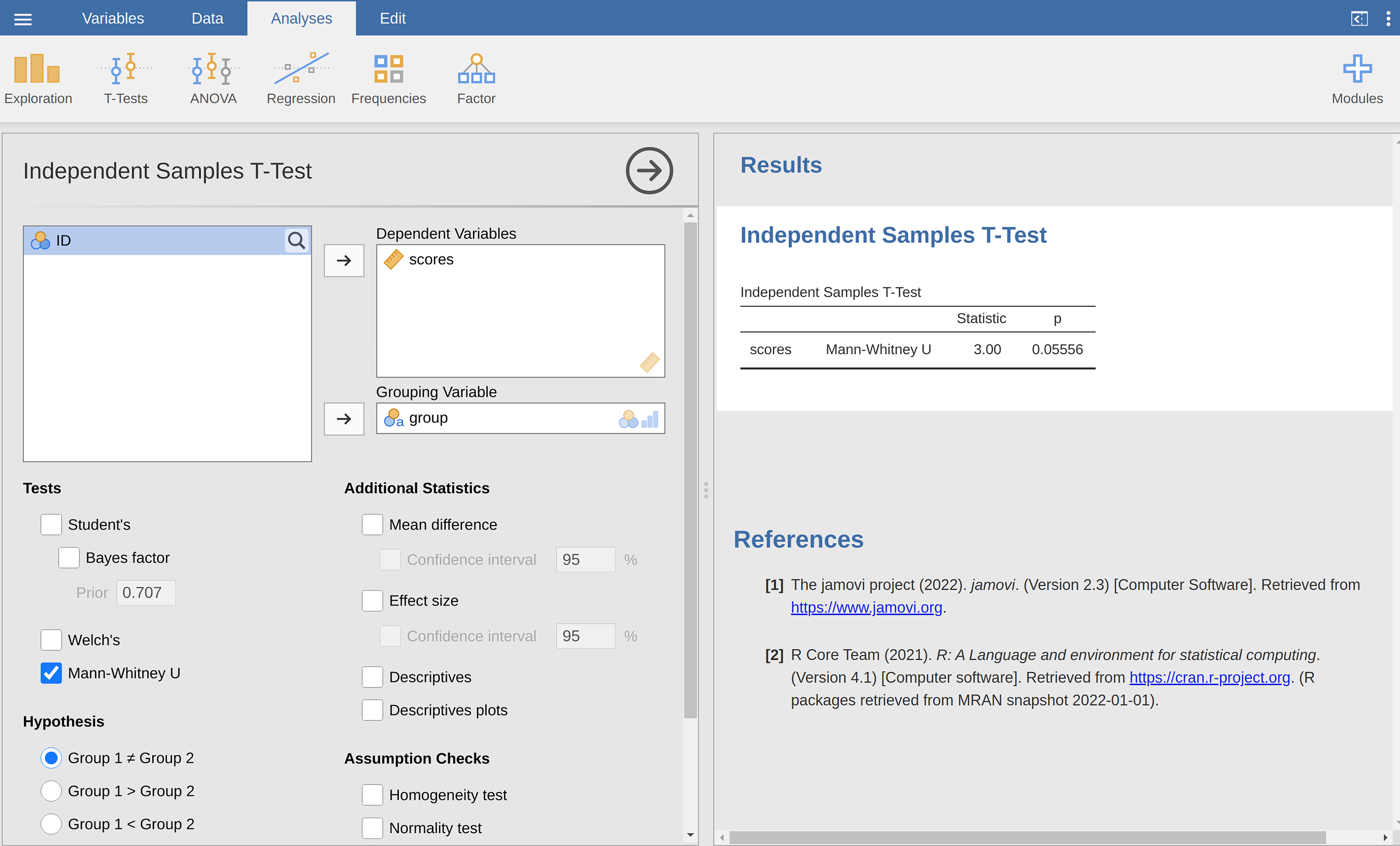
Рис. 122 jamovi screen showing results for the Mann-Whitney U-test

One sample Wilcoxon test

What about the one sample Wilcoxon test (or equivalently, the paired samples Wilcoxon test)? Suppose I am interested in finding out whether taking a statistics class has any effect on the happiness of students. The happiness data set contains the happiness of each student before taking the class and after taking the class . The change score is the difference between the two. Just like we saw with the t-test, there is no fundamental difference between doing a paired-samples test using before and after, versus doing a one-sample test using the change scores. As before, the simplest way to think about the test is to construct a tabulation. The way to do it this time is to take those change scores that are positive differences, and tabulate them against all the complete sample. What you end up with is a table that looks like this:

		all differences
		-24	-14	-10	7	-6	-38	2	-35	-30	5
positive differences	7 2 5				✓	✓		✓ ✓ ✓			✓ ✓

As far as running it in jamovi goes, it is pretty much what you would expect. For the one-sample version, you specify the Wilcoxon rank option under Tests in the One Sample *t*-Test options panel. This gives you Wilcoxon W = 7, p-value = 0.0371. As this shows, we have a significant effect. Evidently, taking a statistics class does have an effect on your happiness. Switching to a paired samples version of the test will not give us a different answer, of course; see Рис. 123.[2]

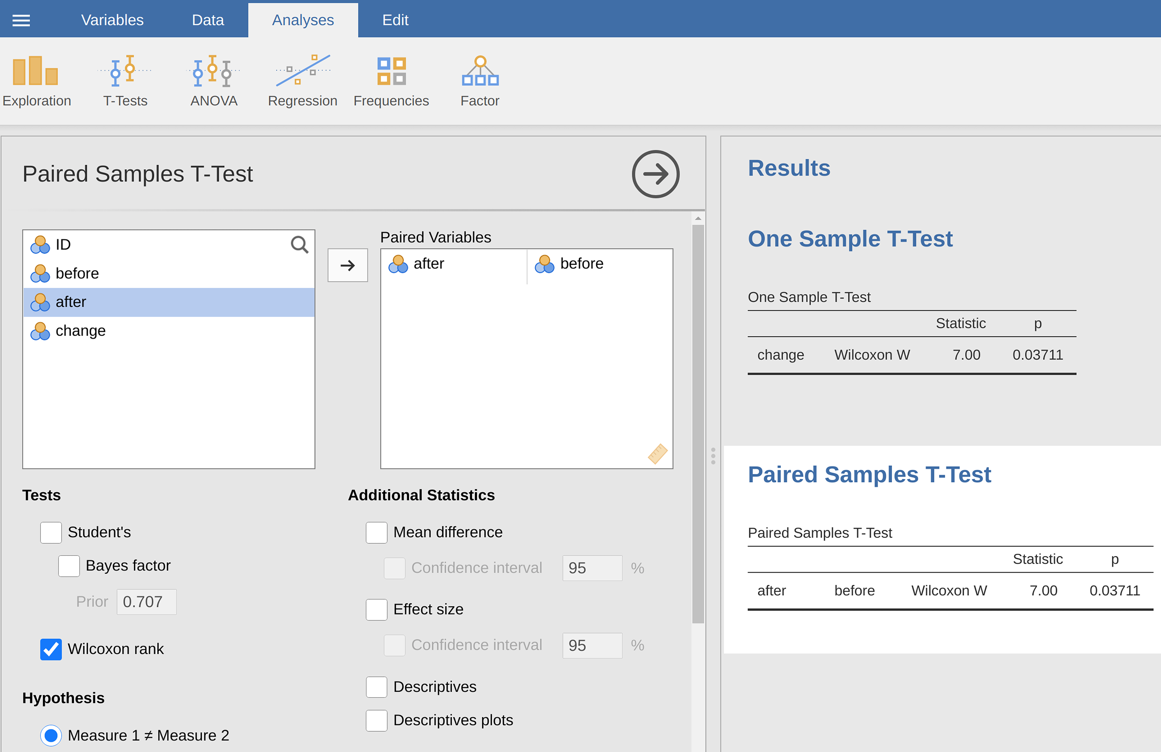
Рис. 123 jamovi screen showing results for one sample and paired sample Wilcoxon non-parametric tests

---

[1]

Actually, there are two different versions of the test statistic that differ from each other by a constant value. The version that I have described is the one that jamovi calculates.

[2]

The p-value = 0.0371 will be the same regardless of how we arrange the variables. However, the value for W depends on the order in which the variables are arranged in the variable pairs. It is also W = 7 if after is put in as the first variable in the pair, but it is W = 48 if before is put in as the first variable in the pair. Adding up 7 and 48 gives us 55 which is the sum of ranks for N = 10 (1 + 2 … + 10). This indicates that the distance from the mean rank = 27.5 is decisive, which is 20.5 in either case (27.5 - 7 or 48 - 27.5).