Autore della sezione: Danielle J. Navarro and David R. Foxcroft

ANOVA as a linear model

One of the most important things to understand about ANOVA and regression is that they are basically the same thing. On the surface of it, you maybe would not think this is true. After all, the way that I have described them so far suggests that ANOVA is primarily concerned with testing for group differences, and regression is primarily concerned with understanding the correlations between variables. And, as far as it goes that is perfectly true. But when you look under the hood, so to speak, the underlying mechanics of ANOVA and regression are awfully similar. In fact, if you think about it, you have already seen evidence of this. ANOVA and regression both rely heavily on sums of squares (SS), both make use of F-tests, and so on. Looking back, it is hard to escape the feeling that chapters Correlation and linear regression and Comparing several means (one-way ANOVA) were a bit repetitive.

The reason for this is that ANOVA and regression are both kinds of linear models. In the case of regression, this is kind of obvious. The regression equation that we use to define the relationship between predictors and outcomes is the equation for a straight line, so it is quite obviously a linear model, with the equation:

Y_p = b₀ + b₁ X_1p + b₂ X_2p + ϵ_p

Y_p is the outcome value for the p-th observation (e.g., p-th person), X_1p is the value of the first predictor for the p-th observation, X_2p is the value of the second predictor for the p-th observation, the b₀, b₁, and b₂ terms are our regression coefficients, and ϵ_p is the p-th residual. If we ignore the residuals ϵ_p and just focus on the regression line itself, we get the following formula:

Ŷ_p = b₀ + b₁ X_1p + b₂ X_2p

where Ŷ_p is the value of Y that the regression line predicts for person p, as opposed to the actually-observed value Y_p. It is not immediately obvious is that we can write ANOVA as a linear model as well, but it is actually pretty straightforward to do this.

Some data

To make things concrete, let us suppose that our outcome variable is the grade that a student receives in my class, a ratio-scale variable corresponding to a mark from 0% to 100%. There are two predictor variables of interest: whether or not the student turned up to lectures (the attend variable) and whether or not the student actually read the textbook (the reading variable). We will say that attend = 1 if the student attended class, and attend = 0 if they did not. Similarly, we will say that reading = 1 if the student read the textbook, and reading = 0 if they did not.

For the purposes of this example, let Y_p denote the grade of the p-th student in the class. This is not quite the same notation that we used earlier in this chapter. Previously, we have used the notation Y_rci to refer to the i-th person in the r-th group for predictor 1 (the row factor) and the c-th group for predictor 2 (the column factor). This extended notation was really handy for describing how the SS values are calculated, but it is a pain in the current context, so I will switch notation here. Now, the Y_p notation is visually simpler than Y_rci, but it has the shortcoming that it does not actually keep track of the group memberships! That is, if I told you that Y_0,0,3 = 35, you would immediately know that we are talking about a student (the 3rd such student, in fact) who did not attend the lectures (i.e., attend = 0) and did not read the textbook (i.e. reading = 0), and who ended up failing the class (grade = 35). But if I tell you that Y_p = 35, all you know is that the p-th student did not get a good grade. We have lost some key information here. What we will do instead is introduce two new variables X_1p and X_2p that keep track of this information. In the case of our hypothetical student, we know that X_1p = 0 (i.e., attend = 0) and X_2p = 0 (i.e., reading = 0). So the data might look like this:

person, p	grade, Yp	attend, X1p	reading, X2p
1	90	1	1
2	87	1	1
3	75	0	1
4	60	1	0
5	35	0	0
6	50	0	0
7	65	1	0
8	70	0	1

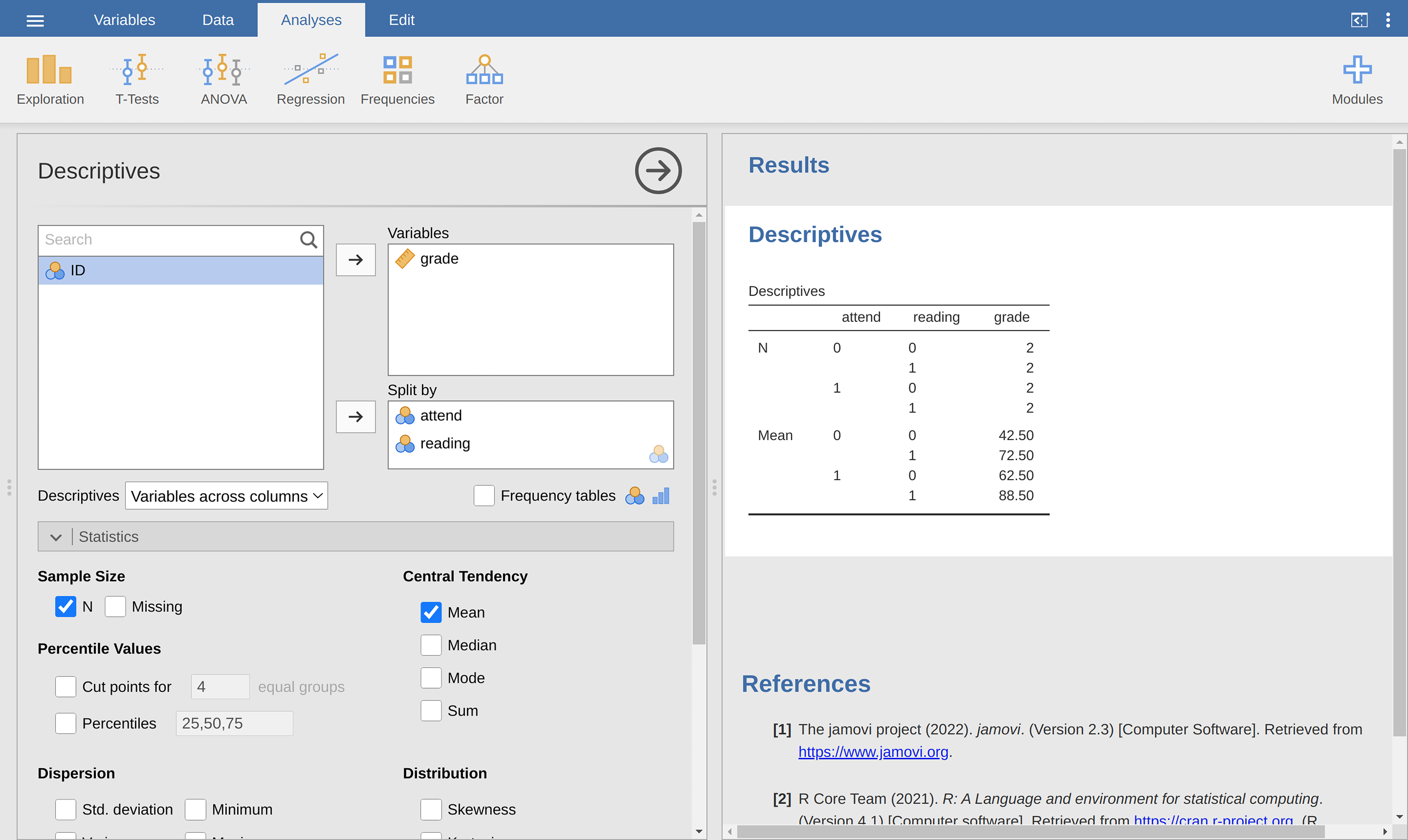
This is not anything particularly special, of course. It is exactly the format in which we expect to see our data! See the rtfm data set. We can use the jamovi analysis Descriptives to confirm that this data set corresponds to a balanced design, with two observations for each combination of attend and reading. In the same way we can also calculate the mean grade for each combination. This is shown in Fig. 181. Looking at the mean scores, one gets the strong impression that reading the text and attending the class both matter a lot.

Fig. 181 jamovi descriptives for the rtfm data set

ANOVA with binary factors as a regression model

Okay, let us get back to talking about the mathematics. We now have our data expressed in terms of three numeric variables: the continuous variable Y and the two binary variables X₁ and X₂. What I want you to recognise is that our 2 × 2 factorial ANOVA is exactly equivalent to the regression model:

Y_p = b₀ + b₁ X_1p + b₂ X_2p + ϵ_p

This is, of course, the exact same equation that I used earlier to describe a two-predictor regression model! The only difference is that X₁ and X₂ are now binary variables (i.e., values can only be 0 or 1), whereas in a regression analysis we expect that X₁ and X₂ will be continuous. There is a couple of ways I could try to convince you of this. One possibility would be to do a lengthy mathematical exercise proving that the two are identical. However, I am going to go out on a limb and guess that most of the readership of this book will find that annoying rather than helpful. Instead, I will explain the basic ideas and then rely on jamovi to show that ANOVA analyses and regression analyses are not just similar, they are identical for all intents and purposes. Let us start by running this as an ANOVA. To do this, we will use the rtfm data set, and Fig. 182 shows what we get when we run the analysis in jamovi.

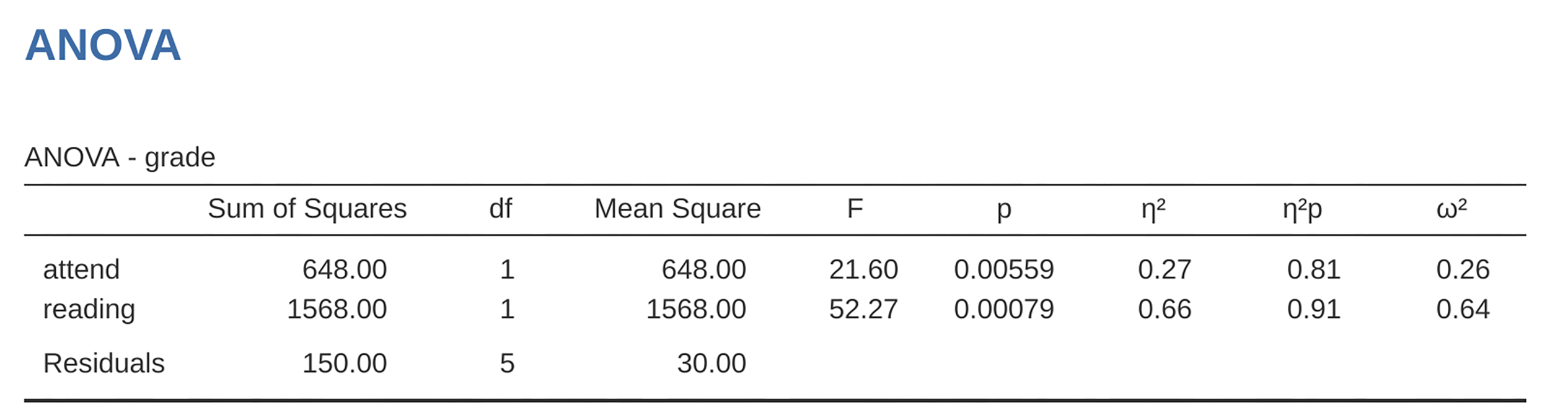
Fig. 182 ANOVA of the rtfm data set in jamovi: Model with two factors attend and reading but without the interaction term for these two factors

So, by reading the key numbers off the ANOVA table and the mean scores that we presented earlier, we can see that the students obtained a higher grade if they attended class (F(1,5) = 21.6, p = 0.0056) and if they read the textbook: F(1,5) = 52.3,*p* = 0.0008. Let us make a note of those p-values and those F-statistics.

Now let us think about the same analysis from a linear regression perspective. In the rtfm data set, we have encoded attend and reading as if they were numeric predictors: A student who turned up to class (i.e., attend = 1) had “more attendance” than a student who did not (i.e., attend = 0). So it is not at all unreasonable to include it as a predictor in a regression model. It is a little unusual, because the predictor only takes on two possible values, but it does not violate any assumption of linear regression. And it is easy to interpret. If the regression coefficient for attend is greater than 0 it means that students that attend lectures get higher grades. If it is less than zero then students attending lectures get lower grades. The same is true for our reading variable.

Why is this true? It is something that is intuitively obvious to everyone who has taken a few statistics classes and is comfortable with the maths, but it is not clear to everyone else at first pass. To see why this is true, it helps to look closely at a few specific students. Let us start by considering the sixth and seventh students in our data set (i.e., p = 6 and p = 7). Neither of them has read the textbook, so in both cases we can set reading = 0. Or, in our mathematical notation, X_2,6 = 0 and X_2,7 = 0. However, student 7 did turn up to lectures (i.e., attend = 1, X_1,7 = 1) whereas student 6 did not (i.e., attend = 0, X_1,6 = 0). When we insert these numbers into the general formula for our regression line, for student 6, the regression predicts that:

Ŷ₆ = b₀ + b₁ X_1,6 + b₂ X_2,6

Ŷ₆ = b₀ + b₁ · 0 + b₂ · 0

Ŷ₆ = b₀

So we are expecting that this student will obtain a grade corresponding to the value of the intercept term b₀. When we insert the numbers for student 7 into the formula for the regression line, we obtain the following:

Ŷ₇ = b₀ + b₁ X_1,7 + b₂ X_2,7

Ŷ₇ = b₀ + b₁ · 1 + b₂ · 0

Ŷ₇ = b₀ + b₁

Because this student attended class, the predicted grade is equal to the intercept term b₀ plus the coefficient associated with the attend variable, b₁. So, if b₁ is greater than zero, we are expecting that the students who turned up to lectures will get higher grades than those students who did not. If this coefficient is negative we are expecting the opposite: students who turn up at class end up performing much worse. In fact, we can push this a little bit further. For student 1, who turned up to class (X_1,1 = 1) and read the textbook (X_2,1 = 1), the regression predicts:

Ŷ₁ = b₀ + b₁ X_1,1 + b₂ X_2,1

Ŷ₁ = b₀ + b₁ · 1 + b₂ · 1

Ŷ₁ = b₀ + b₁ + b₂

So if we assume that attending class helps you get a good grade (i.e., b₁ > 0) and if we assume that reading the textbook also helps you get a good grade (i.e., b₂ > 0), then our expectation is that student 1 will get a grade that that is higher than student 6 and student 7.

And at this point you will not be at all suprised to learn that the regression model predicts that student 3, who read the book but did not attend lectures, will obtain a grade of b₂ + b₀. I will not bore you with yet another regression formula. Instead, what I will do is show you the following table of expected grades:

		read the textbook?
		no	yes
attended?	no	b0	b0 + b2
	yes	b0 + b1	b0 + b1 + b2

As you can see, the intercept term b₀ acts like a kind of “baseline” grade that you would expect from those students who do not take the time to attend class or read the textbook. Similarly, b₁ represents the boost that you are expected to get if you come to class, and b₂ represents the boost that comes from reading the textbook. In fact, if this were an ANOVA you might very well want to characterise b₁ as the main effect of attendance, and b₂ as the main effect of reading! In fact, for a simple 2 × 2 ANOVA that is exactly how it plays out.

We are really starting to see why ANOVA and regression are basically the same thing. When using the rtfm data set with the jamovi regression analysis, we obtain the results shown in Fig. 183.

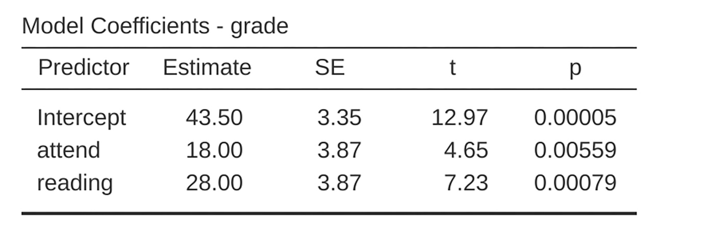
Fig. 183 Regression analysis for the rtfm data set in jamovi: Model with two factors attend and reading but without the interaction term for these two factors

There is a few interesting things to note. First, notice that the intercept term is 43.5 which is close to the “group” mean of 42.5 observed for those two students who did not read the text or attend class. Second, notice that we have the regression coefficient of b₁ = 18.0 for the variable attend, suggesting that those students who attended class scored 18% higher than those who did not. So our expectation would be that those students who turned up to class but did not read the textbook would obtain a grade of b₀ + b₁, which is equal to 43.5 + 18.0 = 61.5. You can verify for yourself that the same thing happens when we look at the students that read the textbook.

Actually, we can push a little further in establishing the equivalence of our ANOVA and our regression. Look at the p-values associated with the attend variable and the reading variable in the regression output. They are identical to the ones we encountered earlier when running the ANOVA. This might seem a little surprising, since the test used when running our regression model calculates a t-statistic and the ANOVA calculates an F-statistic. However, if you can remember all the way back to chapter Introduction to probability, I mentioned that there is a relationship between the t-distribution and the F-distribution. If you have some quantity that is distributed according to a t-distribution with k degrees of freedom and you square it, then this new squared quantity follows an F-distribution whose degrees of freedom are 1 and k. We can check this with respect to the t-statistics in our regression model. For the attend variable we get a t-value of 4.65. If we square this number we end up with 21.6, which matches the corresponding F-statistic in our ANOVA.

Finally, one last thing you should know. Because jamovi understands the fact that ANOVA and regression are both examples of linear models, it lets you extract the classic ANOVA table from your regression model using the Linear Regression → Model Coefficients → Omnibus Test → ANOVA test, and this will give you the table shown in Fig. 184.

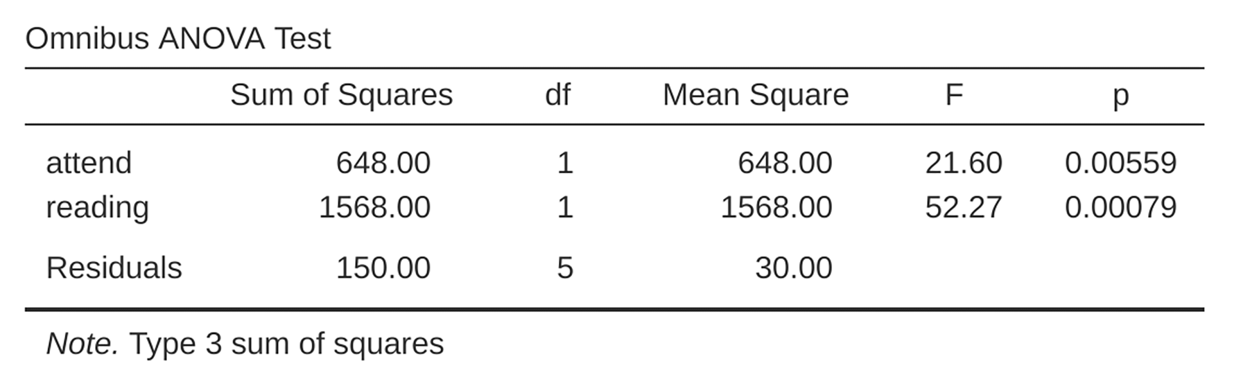
Fig. 184 Results table showing the Omnibus ANOVA Test from the jamovi regression analysis using the rtfm data set

How to encode non-binary factors as contrasts

At this point, I have shown you how we can view a 2 × 2 ANOVA into a linear model. And it is pretty easy to see how this generalises to a 2 × 2 × 2 ANOVA or a 2 × 2 × 2 × 2 ANOVA. It is the same thing, really. You just add a new binary variable for each of your factors. Where it begins to get trickier is when we consider factors that have more than two levels. Consider, for instance, the 3 × 2 ANOVA that we ran earlier in this chapter using the clinicaltrial data set. How can we convert the three-level drug factor into a numerical form that is appropriate for a regression?

The answer to this question is pretty simple, actually. All we have to do is realise that a three-level factor can be redescribed as two binary variables. Suppose, for instance, I were to create a new binary variable called druganxifree. Whenever the drug variable is equal to anxifree we set druganxifree = 1. Otherwise, we set druganxifree = 0. This variable sets up a contrast, in this case between anxifree and the other two drugs. By itself, of course, the druganxifree contrast is not enough to fully capture all of the information in our drug variable. We need a second contrast, one that allows us to distinguish between joyzepam and the placebo. To do this, we can create a second binary contrast, called drugjoyzepam, which equals 1 if the drug is joyzepam and 0 if it is not. Taken together, these two contrasts allows us to perfectly discriminate between all three possible levels of drug. The table below illustrates this:

drug	druganxifree	drugjoyzepam
placebo	0	0
anxifree	1	0
joyzepam	0	1

If the drug administered to a patient is a placebo then both of the two contrast variables will equal 0. If the drug is anxifree then the druganxifree variable will equal 1, and drugjoyzepam will be 0. The reverse is true for joyzepam: drugjoyzepam is 1 and druganxifree is 0.

Creating contrast variables is not too difficult to do using the jamovi Compute command to create a new variable. For example, to create the druganxifree variable, write this logical expression in the formula box: IF(drug == 'anxifree', 1, 0). Similarly, to create the new variable drugjoyzepam use this logical expression: IF(drug == 'joyzepam', 1, 0). Likewise for therapyCBT: IF(therapy == 'CBT', 1, 0). You can see these new variables, and the corresponding logical expressions, in the clinicaltrial2 data set.

We have now recoded our three-level factor in terms of two binary variables, and we have already seen that ANOVA and regression behave the same way for binary variables. However, there are some additional complexities that arise in this case, which we will discuss in the next section.

The equivalence between ANOVA and regression for non-binary factors

Now we have two different versions of the same data set. Our original data in which the drug variable from the clinicaltrial data set is expressed as a single three-level factor, and the clinicaltrial2 data set in which it is expanded into two binary contrasts. Once again, the thing that we want to demonstrate is that our original 3 × 2 factorial ANOVA is equivalent to a regression model applied to the contrast variables. Let us start by re-running the ANOVA, with results shown in Fig. 185.

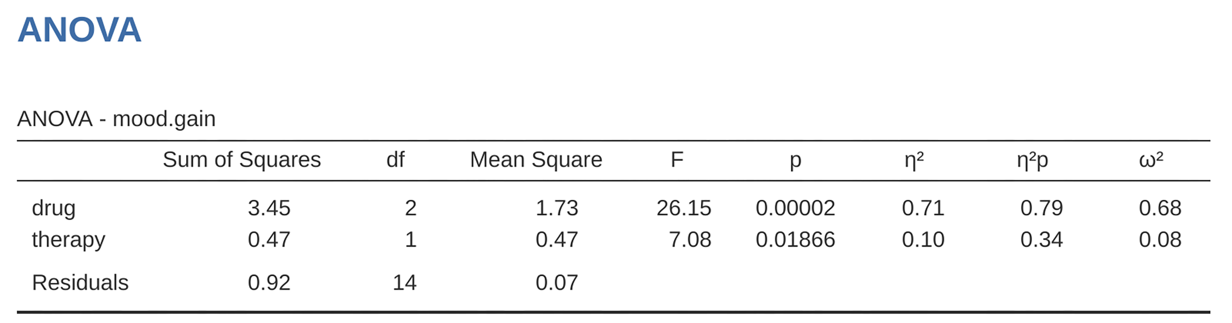
Fig. 185 jamovi ANOVA results for the clinicaltrial data set: Unsaturated model with the two main effects for drug and therapy but without an interaction component for these two factors

Obviously, there are no surprises here. That is the exact same ANOVA that we ran earlier. Next, let us run a regression using druganxifree, drugjoyzepam and therapyCBT as the predictors. The results are shown in Fig. 186.

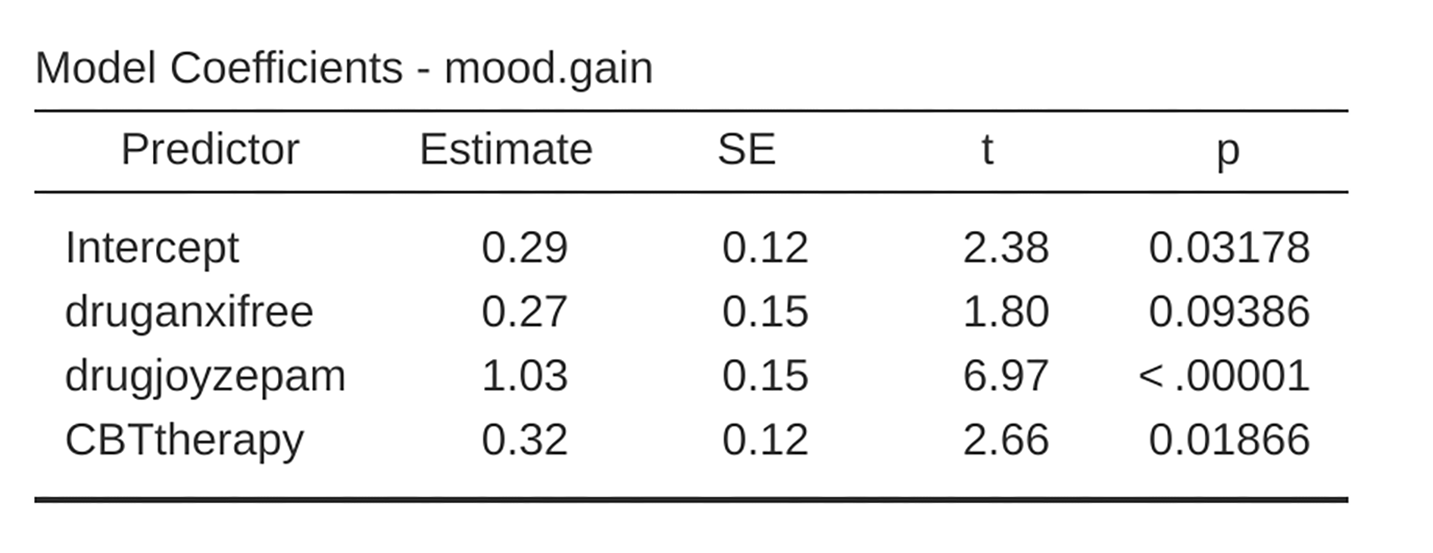
Fig. 186 jamovi regression results for the clinicaltrial data set: Model with the generated contrast variables druganxifree and drugjoyzepam

However, this is not the same output that we got last time. Not surprisingly, the regression output prints out the results for each of the three predictors separately, just like it did every other time we conducted a regression analysis. On the one hand we can see that the p-value for the therapyCBT variable is exactly the same as the one for the therapy factor in our original ANOVA, so we can be reassured that the regression model is doing the same thing as the ANOVA did. On the other hand, this regression model is testing the druganxifree contrast and the drugjoyzepam contrast separately, as if they were two completely unrelated variables. It is not surprising, because the poor regression analysis has no way of knowing that drugjoyzepam and druganxifree are actually the two different contrasts that we used to encode our three-level drug factor. As far as it knows, drugjoyzepam and druganxifree are no more related to one another than drugjoyzepam and therapyCBT. However, we are not at all interested in determining whether these two contrasts are individually significant. We just want to know if there is an “overall” effect of drug. That is, what we want jamovi to do is to run some kind of “model comparison” test, one in which the two “drug-related” contrasts are lumped together for the purpose of the test. All we need to do is specify our null model, which in this case would include the therapyCBT predictor, and omit both of the drug-related variables, as in Fig. 187.

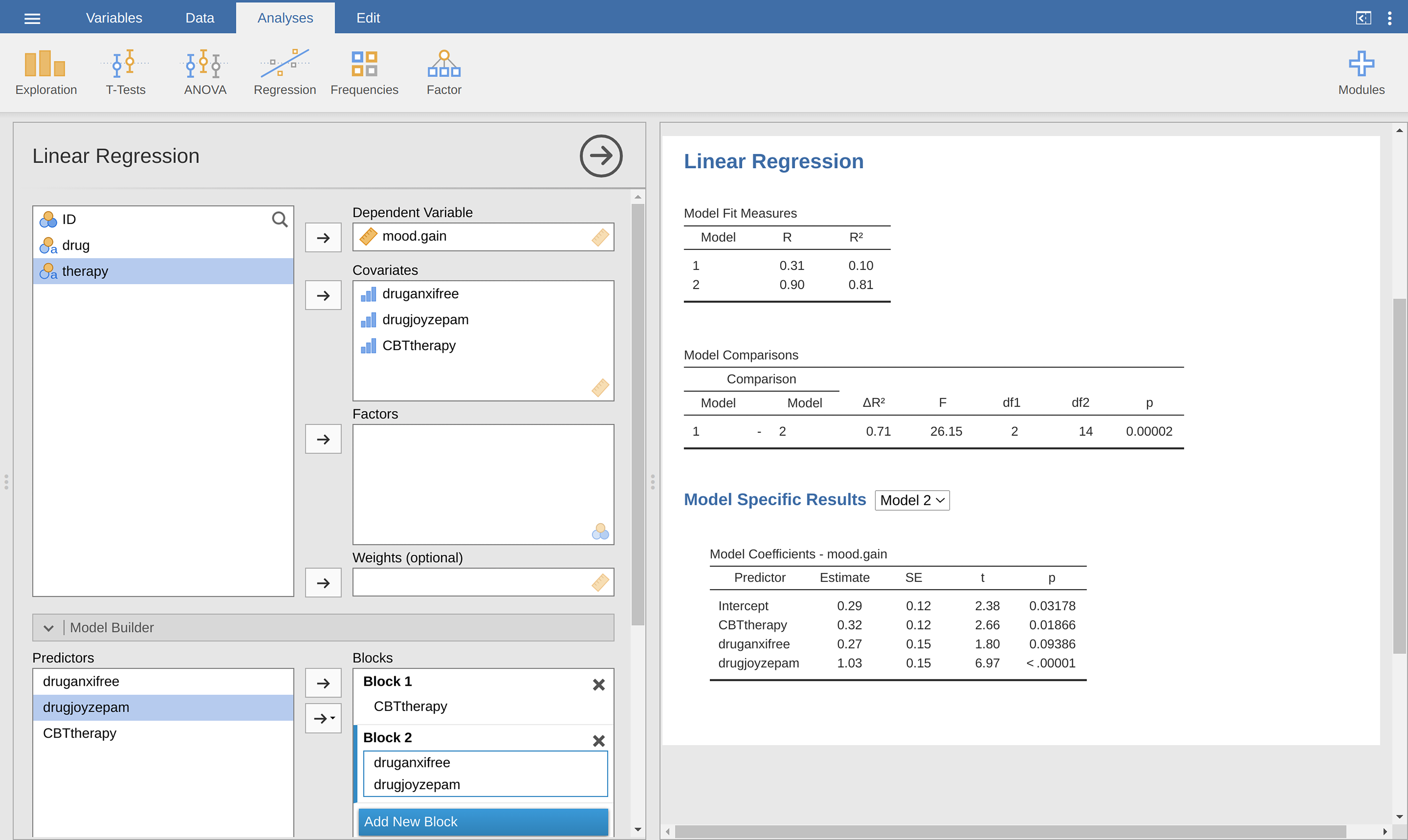
Fig. 187 Model comparison in jamovi regression: Null model (Model 1) vs. model using the generated contrast variables (Model 2)

Our F-statistic is 26.15, the degrees of freedom are 2 and 14, and the p-value is 0.00002. The numbers are identical those we obtained for the main effect of drug in our original ANOVA. Once again we see that ANOVA and regression are essentially the same. They are both linear models, and the underlying statistical machinery for ANOVA is identical to the machinery used in regression. The importance of this fact should not be understated. Throughout the rest of this chapter we are going to rely heavily on this idea.

Although we went through all the faff of computing new variables in jamovi for the contrasts druganxifree and drugjoyzepam, just to show that ANOVA and regression are essentially the same, in the jamovi linear regression analysis there is actually a nifty shortcut to get these contrasts, see Fig. 188. What jamovi is doing here is allowing you to enter categorical predictor variables as factors! You can also specify which group to use as the reference level, via the Reference Levels option. We have changed this to placebo and no.therapy, respectively, because this makes most sense.

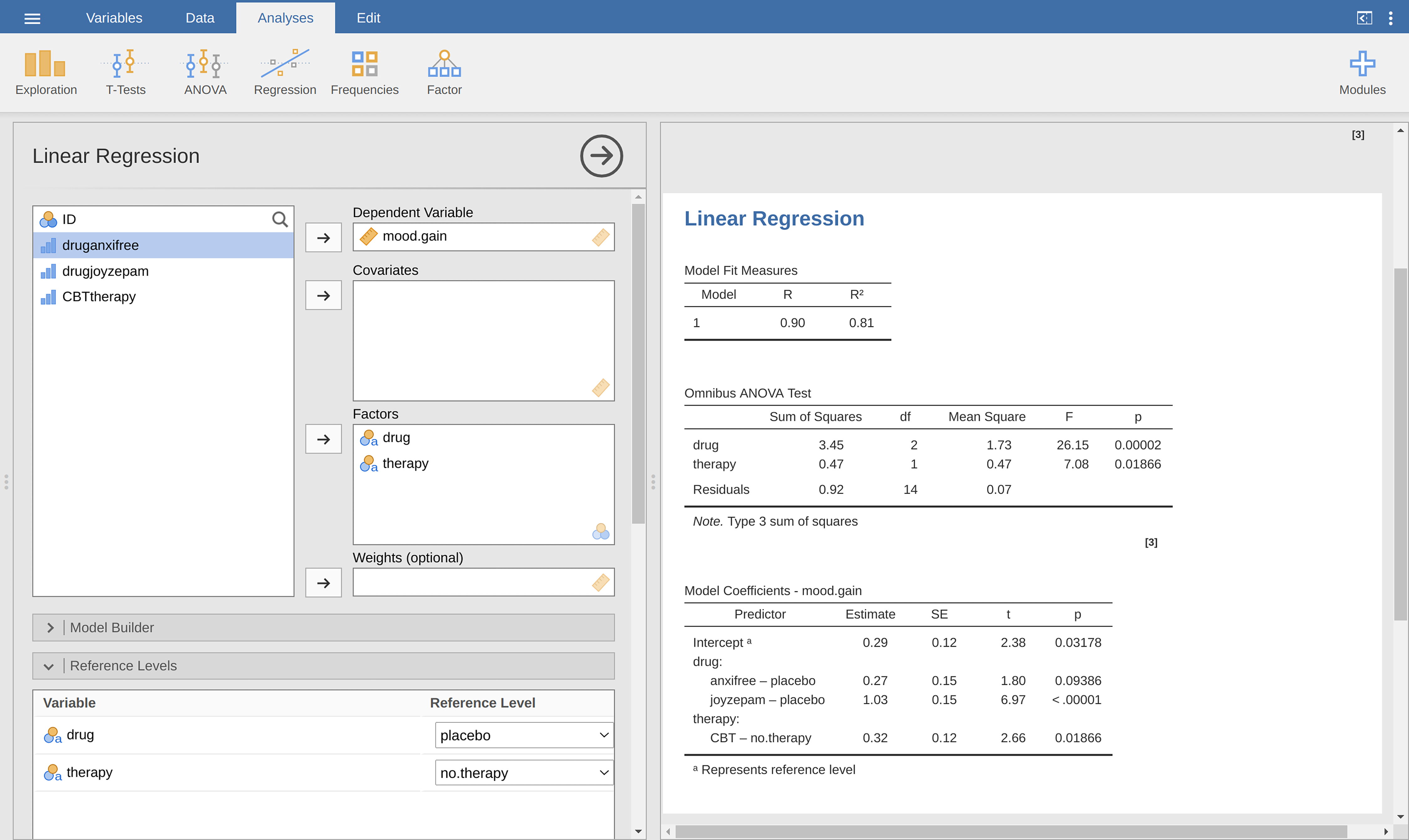
Fig. 188 Regression analysis with factors and contrasts in jamovi, including omnibus ANOVA test results

If you also set the ANOVA test checkbox under the Model Coefficients → Omnibus Test option, we see that the F-statistic is 26.15, the degrees of freedom are 2 and 14, and the p-value is 0.00002 (see Fig. 188). The numbers are identical to the ones we obtained for the main effect of drug in our original ANOVA. Once again, we see that ANOVA and regression are essentially the same. They are both linear models, and the underlying statistical machinery for ANOVA and for regression is identical.

Degrees of freedom as parameter counting!

At long last, I can finally give a definition of degrees of freedom that I am happy with. Degrees of freedom are defined in terms of the number of parameters that have to be estimated in a model. For a regression model or an ANOVA, the number of parameters corresponds to the number of regression coefficients (i.e., the b-values), including the intercept. Keeping in mind that any F-test is always a comparison between two models and the first df is the difference in the number of parameters. For example, in the model comparison above, the null model (mood.gain ~ therapyCBT) has two parameters: there is one regression coefficient for the therapyCBT variable, and a second one for the intercept. The alternative model (mood.gain ~ druganxifree + drugjoyzepam + therapyCBT) has four parameters: one regression coefficient for each of the three contrasts, and one more for the intercept. So the degrees of freedom associated with the difference between these two models is df₁ = 4 - 2 = 2.

What about the case when there does not seem to be a null model? For instance, you might be thinking of the F-test that shows up when you select F Test under the Linear Regression → Model Fit options. I originally described that as a test of the regression model as a whole. However, that is still a comparison between two models. The null model is the trivial model that only includes one regression coefficient, for the intercept term. The alternative model contains K + 1 regression coefficients, one for each of the K predictor variables and one more for the intercept. So the df-value that you see in this F-test is equal to df₁ = K + 1 - 1 = K.

What about the second df-value that appears in the F-test? This always refers to the degrees of freedom associated with the residuals. It is possible to think of this in terms of parameters too, but in a slightly counter-intuitive way. Think of it like this. Suppose that the total number of observations across the study as a whole is N. If you wanted to perfectly describe each of these N values, you need to use, well… N numbers. When you build a regression model, what you are really doing is specifying that some of the numbers need to perfectly describe the data. If your model has K predictors and an intercept, then you have specified K + 1 numbers. So, without bothering to figure out exactly how this would be done, how many more numbers do you think are going to be needed to transform a K + 1 parameter regression model into a perfect re-description of the raw data? If you found yourself thinking that (K + 1) + (N - K - 1) = N, and so the answer would have to be N - K - 1, well done! That is exactly right. In principle you can imagine an absurdly complicated regression model that includes a parameter for every single data point, and it would of course provide a perfect description of the data. This model would contain N parameters in total, but we are interested in the difference between the number of parameters required to describe this full model (i.e., N) and the number of parameters used by the simpler regression model that you are actually interested in (i.e., K + 1), and so the second degrees of freedom in the F-test is df₂ = N - K - 1, where K is the number of predictors (in a regression model) or the number of contrasts (in an ANOVA). In the example I gave above, there are N = 18 observations in the data set and K + 1 = 4 regression coefficients associated with the ANOVA model, so the degrees of freedom for the residuals is df₂ = 18 - 4 = 14.