Autore della sezione: Danielle J. Navarro and David R. Foxcroft
Effect size, sample size and power
In previous sections I have emphasised the fact that the major design principle behind statistical hypothesis testing is that we try to control our Type I error rate. When we fix α = 0.05 we are attempting to ensure that only 5% of true null hypotheses are incorrectly rejected. However, this does not mean that we do not care about Type II errors. In fact, from the researcher’s perspective, the error of failing to reject the null hypothesis when it is actually false is an extremely annoying one. With that in mind, a secondary goal of hypothesis testing is to try to minimise β, the Type II error rate, although we do not usually talk in terms of minimising Type II errors. Instead, we talk about maximising the power of the test. Since power is defined as 1 - β, this is the same thing.
The power function
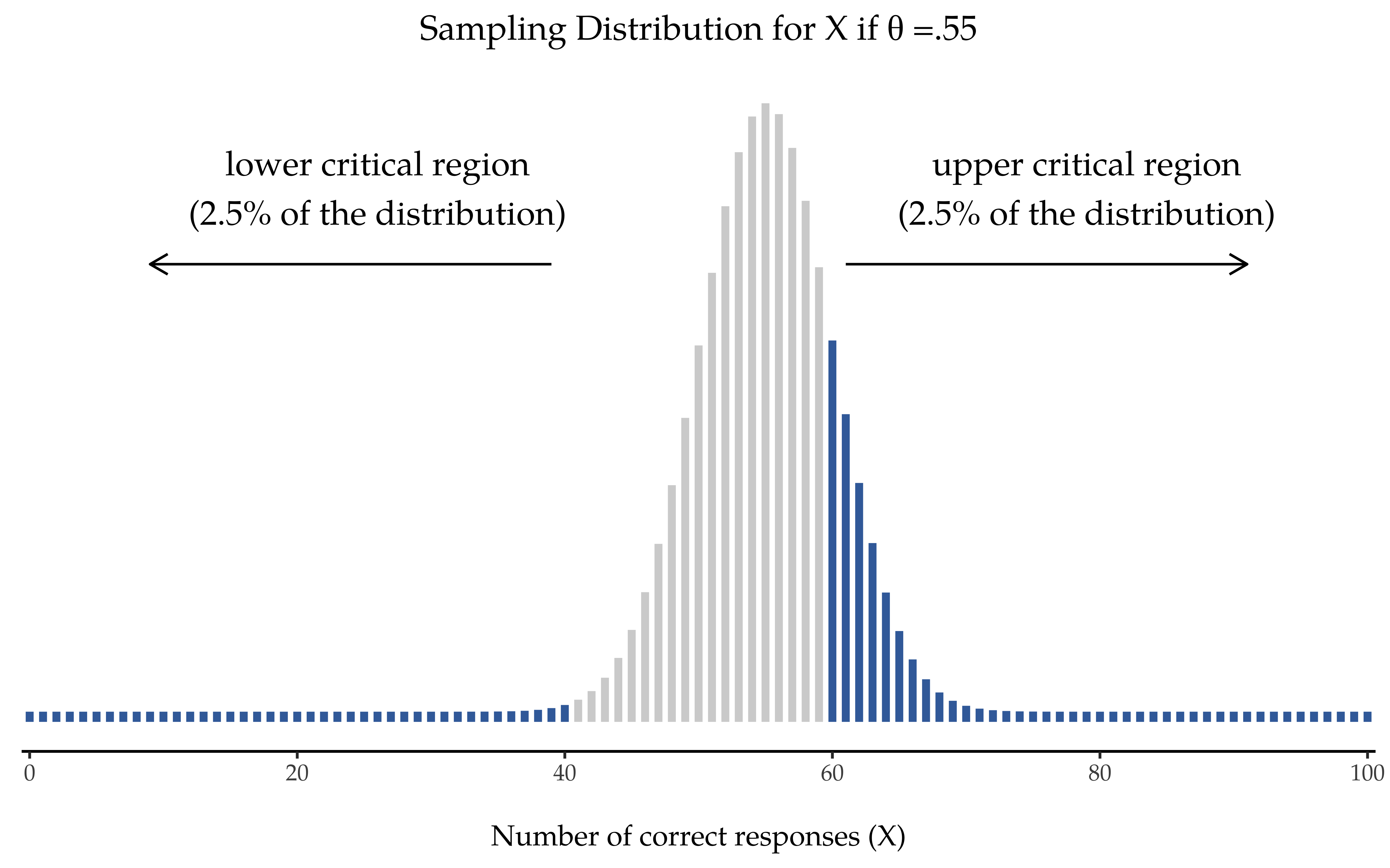
Fig. 85 Sampling distribution under the alternative hypothesis for a population parameter value of θ = 0.55. A reasonable proportion of the distribution lies in the rejection region.
Let us take a moment to think about what a Type II error actually is. A Type II error occurs when the alternative hypothesis is true, but we are nevertheless unable to reject the null hypothesis. Ideally, we would be able to calculate a single number β that tells us the Type II error rate, in the same way that we can set α = 0.05 for the Type I error rate. Unfortunately, this is a lot trickier to do. To see this, notice that in my ESP study the alternative hypothesis actually corresponds to lots of possible values of θ. In fact, the alternative hypothesis corresponds to every value of θ except 0.5. Let us suppose that the true probability of someone choosing the correct response is 55% (i.e., θ = 0.55). If so, then the true sampling distribution for X is not the same one that the null hypothesis predicts, as the most likely value for X is now 55 out of 100. Not only that, the whole sampling distribution has now shifted, as shown in Fig. 85. The critical regions, of course, do not change. By definition the critical regions are based on what the null hypothesis predicts, but when the null hypothesis is wrong, a much larger proportion of the sampling distribution distribution falls in the critical region. And of course that is what should happen. The probability of rejecting the null hypothesis is larger when the null hypothesis is actually false! However θ = 0.55 is not the only possibility consistent with the alternative hypothesis. Let us instead suppose that the true value of θ is actually 0.70. What happens to the sampling distribution when this occurs? The answer, shown in Fig. 86, is that almost the entirety of the sampling distribution has now moved into the critical region. Therefore, if θ = 0.70, the probability of us correctly rejecting the null hypothesis (i.e., the power of the test) is much larger than if θ = 0.55. In short, while θ = 0.55 and θ = 0.70 are both part of the alternative hypothesis, the Type II error rate is different.
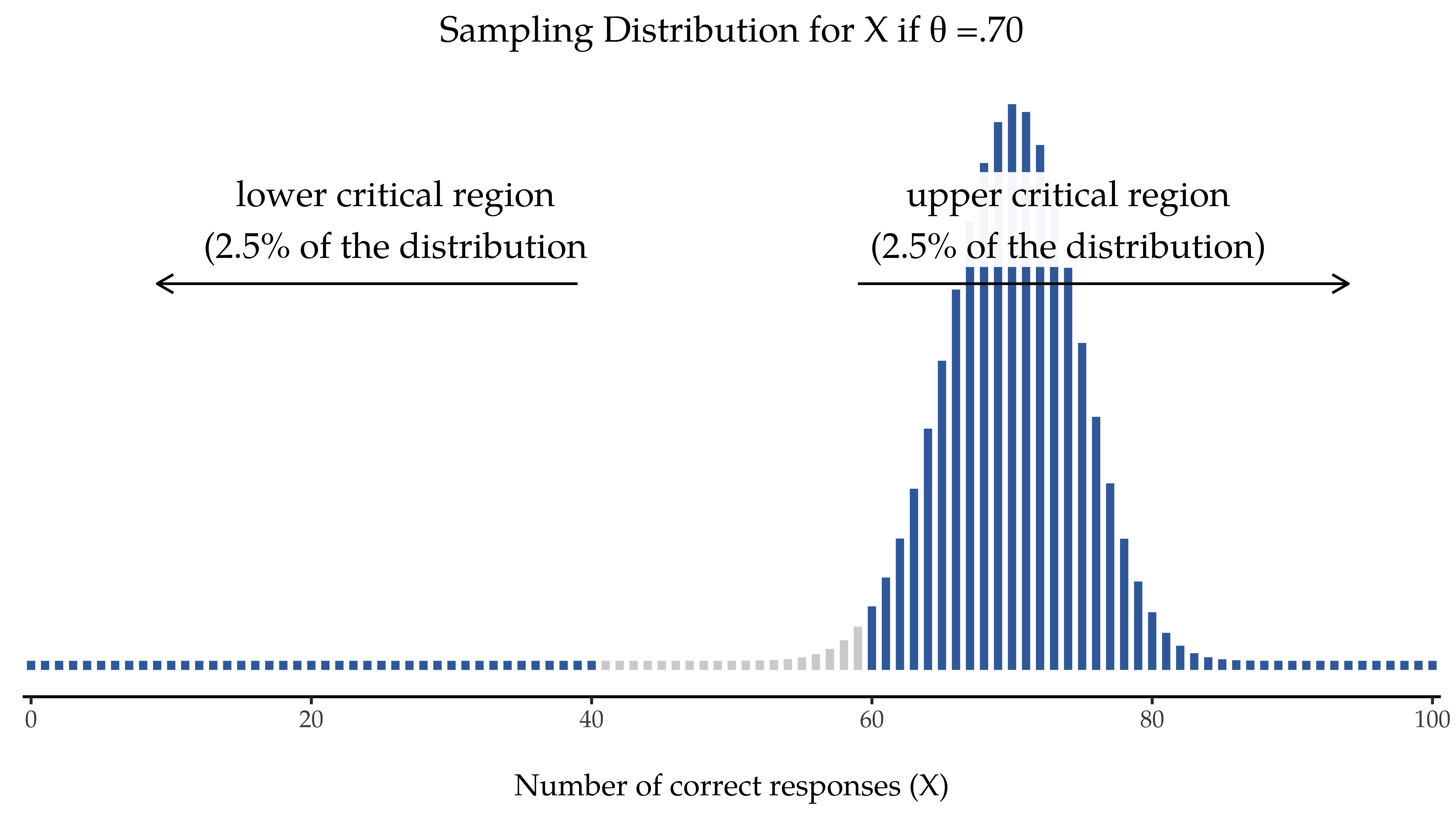
Fig. 86 Sampling distribution under the alternative hypothesis for a population parameter value of θ = 0.70. Almost all of the distribution lies in the rejection region.
What all this means is that the power of a test (i.e., 1 - β) depends on the true value of θ. To illustrate this, I have calculated the expected probability of rejecting the null hypothesis for all values of θ, and plotted it in Fig. 87. This plot describes what is usually called the power function of the test. It is a nice summary of how good the test is, because it actually tells you the power (1 - β) for all possible values of θ. As you can see, when the true value of θ is very close to 0.5, the power of the test drops very sharply, but when it is further away, the power is large.
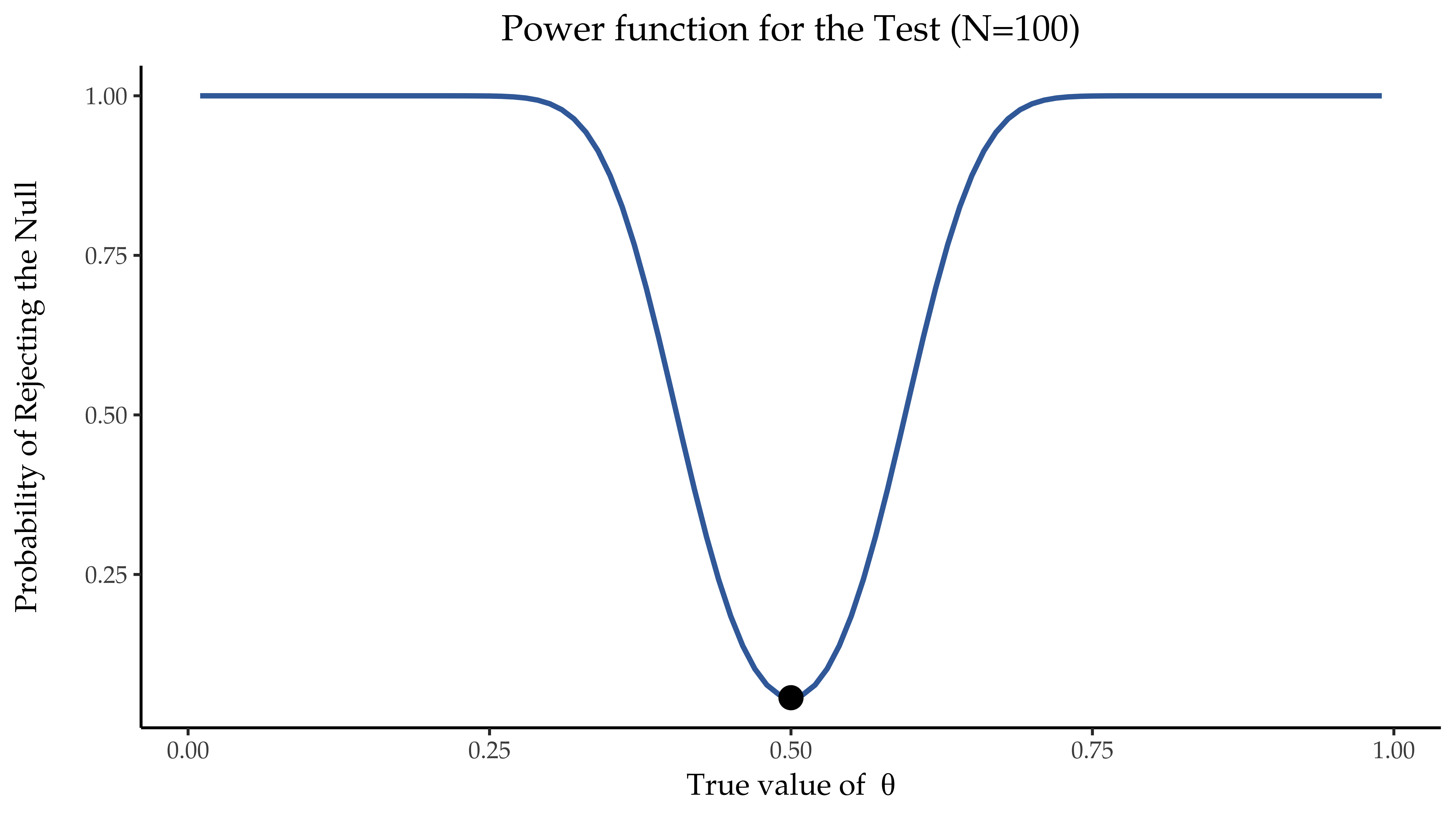
Fig. 87 The probability that we will reject the null hypothesis, plotted as a function of the true value of θ. Obviously, the test is more powerful (greater chance of correct rejection) if the true value of θ is very different from the value that the null hypothesis specifies (i.e., θ = 0.5). Notice that when θ actually is equal to 0.5 (plotted as a black dot), the null hypothesis is in fact true and rejecting the null hypothesis in this instance would be a Type I error.
Effect size
Since all models are wrong the scientist must be alert to what is importantly wrong. It is inappropriate to be concerned with mice when there are tigers abroad
The plot shown in Fig. 87 captures a fairly basic point about hypothesis testing. If the true state of the world is very different from what the null hypothesis predicts then your power will be very high, but if the true state of the world is similar to the null hypothesis (but not identical) then the power of the test is going to be very low. Therefore, it is useful to be able to have some way of quantifying how “similar” the true state of the world is to the null hypothesis. A statistic that does this is called a measure of effect size (Cohen, 1988, Ellis, 2010).
Effect size is defined slightly differently in different contexts (and so this section just talks in general terms) but the qualitative idea that it tries to capture is always the same. How big is the difference between the true population parameters and the parameter values that are assumed by the null hypothesis? In our ESP example, if we let θ0 = 0.5 denote the value assumed by the null hypothesis and let θ denote the true value, then a simple measure of effect size could be something like the difference between the true value and value assumed by the null hypothesis (i.e., θ - θ0), or possibly just the magnitude of this difference, abs(θ - θ0).
big effect size |
small effect size |
|
|---|---|---|
significant result |
difference is real, and of practical importance |
difference is real, but might not be interesting |
non-significant result |
no effect observed |
no effect observed |
Why calculate effect size? Let us assume that you have run your experiment, collected the data, and gotten a significant effect when you ran your hypothesis test. Is it not enough just to say that you have gotten a significant effect? Surely that is the point of hypothesis testing? Well, sort of. Yes, the point of doing a hypothesis test is to try to demonstrate that the null hypothesis is wrong, but that is hardly the only thing we are interested in. If the null hypothesis claimed that θ = 0.50 and we show that it is wrong, we have only really told half of the story. Rejecting the null hypothesis implies that we believe that θ ≠ 0.50, but there is a big difference between θ = 0.51 and θ = 0.80. If we find that θ = 0.80, then not only have we found that the null hypothesis is wrong, it appears to be very wrong. On the other hand, suppose we have successfully rejected the null hypothesis, but it looks like the true value of θ is only 0.51 (this would only be possible with a very large study). Sure, the null hypothesis is wrong but it is not at all clear that we actually care because the effect size is so small. In the context of my ESP study we might still care since any demonstration of real psychic powers would actually be pretty cool,[1] but in other contexts a 1% difference usually is not very interesting, even if it is a real difference. For instance, suppose we are looking at differences in high school exam scores between males and females and it turns out that the female scores are 1% higher on average than the males. If I have got data from thousands of students then this difference will almost certainly be statistically significant, but regardless of how small the p-value is, it is just not very interesting. You would hardly want to go around proclaiming a crisis in boys education on the basis of such a tiny difference would you? It is for this reason that it is becoming more common (slowly, but surely) to report some kind of standard measure of effect size along with the the results of the hypothesis test. The hypothesis test itself tells you whether you should believe that the effect you have observed is real (i.e., not just due to chance), whereas the effect size tells you whether or not you should care.
Increasing the power of your study
Not surprisingly, scientists are fairly obsessed with maximising the power of their experiments. We want our experiments to work and so we want to maximise the chance of rejecting the null hypothesis if it is false. As we have seen, one factor that influences power is the effect size. So the first thing you can do to increase your power is to increase the effect size. In practice, what this means is that you want to design your study in such a way that the effect size gets magnified. For instance, in my ESP study I might believe that psychic powers work best in a quiet, darkened room with fewer distractions to cloud the mind. Therefore, I would try to conduct my experiments in just such an environment. If I can strengthen people’s ESP abilities somehow then the true value of θ will go up[2] and therefore my effect size will be larger. In short, clever experimental design is one way to boost power, because it can alter the effect size.
Unfortunately, it is often the case that even with the best of experimental designs you may have only a small effect. Perhaps, for example, ESP really does exist but even under the best of conditions it is very very weak. Under those circumstances your best bet for increasing power is to increase the sample size. In general, the more observations that you have available, the more likely it is that you can discriminate between two hypotheses. If I ran my ESP experiment with ten participants and seven of them correctly guessed the colour of the hidden card you would not be terribly impressed. But if I ran it with 10 000 participants, and 7 000 of them got the answer right, you would be much more likely to think I had discovered something. In other words, power increases with the sample size. This is illustrated in Fig. 88, which shows the power of the test for a true parameter of θ = 0.70 for all sample sizes N from 1 to 100, where I am assuming that the null hypothesis predicts that θ0 = 0.5.
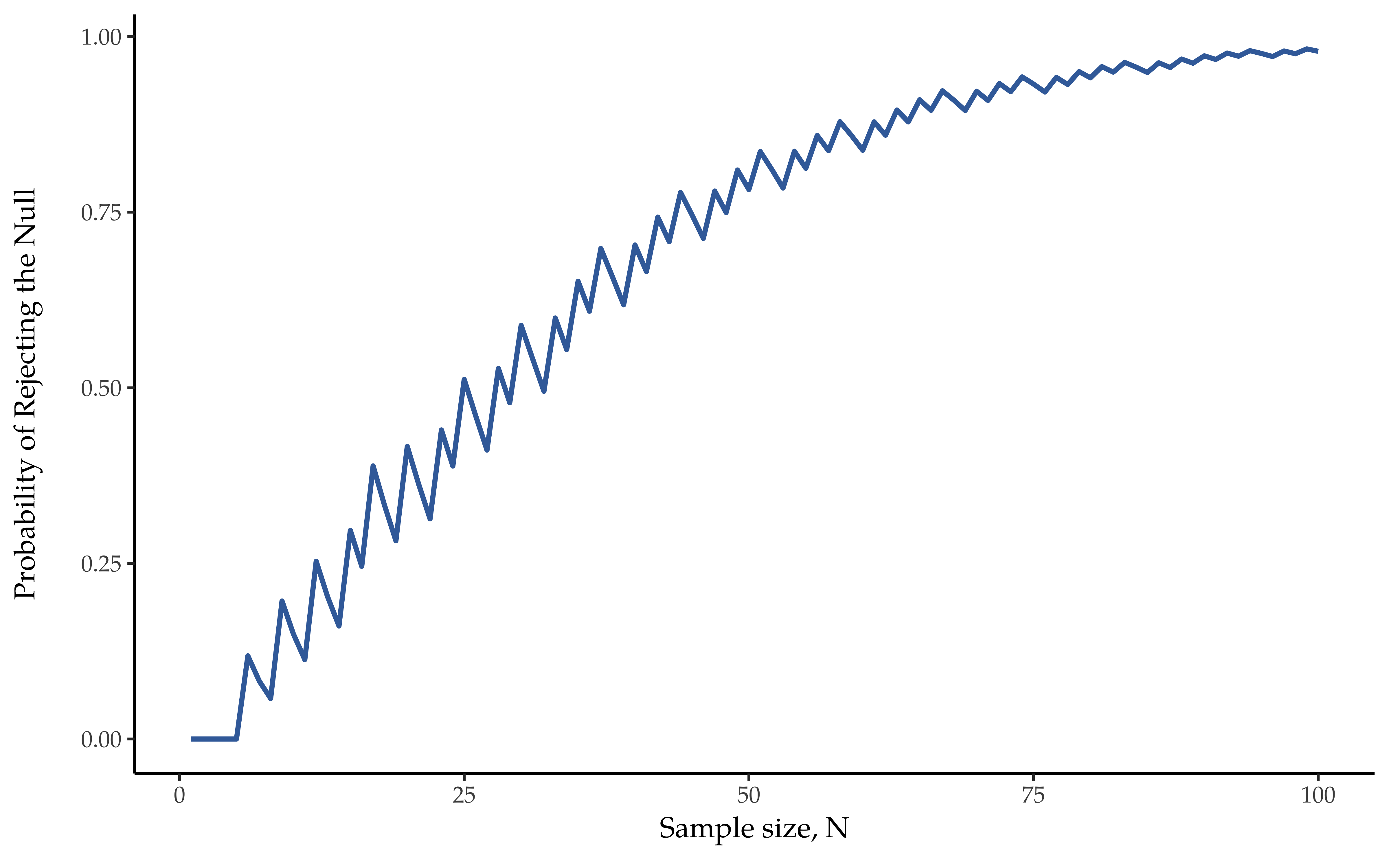
Fig. 88 The power of our test plotted as a function of the sample size N. In this case, the true value of θ is 0.7 but the null hypothesis is that θ = 0.5. Overall, larger N means greater power (the small zig-zags in this function occur because of some odd interactions between θ, α and the fact that the binomial distribution is discrete, it does not matter for any serious purpose).
Because power is important, whenever you are contemplating running an experiment it would be pretty useful to know how much power you are likely to have. It is never possible to know for sure since you can not possibly know what your real effect size is. However, it is often (well, sometimes) possible to guess how big it should be. If so, you can guess what sample size you need! This idea is called power analysis, and if it is feasible to do it then it is very helpful. It can tell you something about whether you have enough time or money to be able to run the experiment successfully. It is increasingly common to see people arguing that power analysis should be a required part of experimental design, so it is worth knowing about. I do not discuss power analysis in this book, however. This is partly for a boring reason and partly for a substantive one. The boring reason is that I have not had time to write about power analysis yet. The substantive one is that I am still a little suspicious of power analysis. Speaking as a researcher, I have very rarely found myself in a position to be able to do one. It is either the case that (a) my experiment is a bit non-standard and I do not know how to define effect size properly, or (b I literally have so little idea about what the effect size will be that I would not know how to interpret the answers. Not only that, after extensive conversations with someone who does statistics consulting for a living (my wife, as it happens), I can not help but notice that in practice the only time anyone ever asks her for a power analysis is when she is helping someone write a grant application. In other words, the only time any scientist ever seems to want a power analysis in real life is when they are being forced to do it by bureaucratic process. It is not part of anyone’s day-to-day work. In short, I have always been of the view that whilst power is an important concept, power analysis is not as useful as people make it sound, except in the rare cases where (a) someone has figured out how to calculate power for your actual experimental design and (b) you have a pretty good idea what the effect size is likely to be.[3] Maybe other people have had better experiences than me, but I have personally never been in a situation where both (a) and (b) were true. Maybe I will be convinced otherwise in the future, and probably a future version of this book would include a more detailed discussion of power analysis, but for now this is about as much as I am comfortable saying about the topic.