Section author: Danielle J. Navarro and David R. Foxcroft
Confirmatory Factor Analysis
So, our attempt to identify underlying latent factors using EFA with carefully selected questions from the personality item pool seemed to be pretty successful. The next step in our quest to develop a useful measure of personality is to check the latent factors we identified in the original EFA with a different sample. We want to see if the factors hold up, if we can confirm their existence with different data. This is a more rigorous check, as we will see. And it’s called Confirmatory Factor Analysis (CFA) as we will, unsuprisingly, be seeking to confirm a pre-specificied latent factor structure.[1]
In CFA, instead of doing an analysis where we see how the data goes together in an exploratory sense, we instead impose a structure, like in Fig. 191, on the data and see how well the data fits our pre-specified structure. In this sense, we are undertaking a confirmatory analysis, to see how well a pre-specified model is confirmed by the observed data.
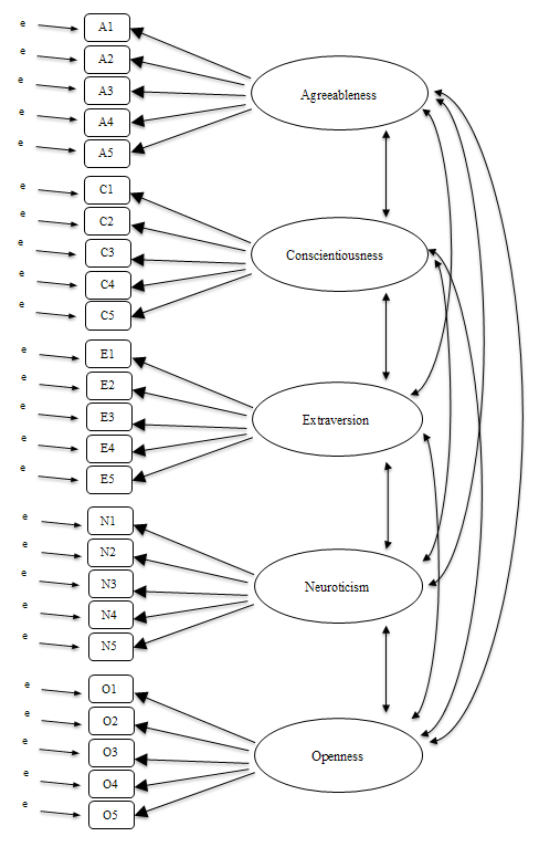
Fig. 191 Initial pre-specification of latent factor structure for the five factor personality scales, for use in CFA
A straightforward confirmatory factor analysis (CFA) of the personality items
would therefore specify five latent factors as shown in Fig. 191,
each measured by five observed variables.
Each variable is a measure of an underlying latent factor. For example, A1
is predicted by the underlying latent factor Agreeableness. And because A1
is not a perfect measure of the Agreeableness factor, there is an error term,
e, associated with it. In other words, e represents the variance in A1
that is not accounted for by the Agreeableness factor. This is sometimes called
measurement error.
The next step is to consider whether the latent factors should be allowed to correlate in our model. As mentioned earlier, in the psychological and behavioural sciences constructs are often related to each other, and we also think that some of our personality factors may be correlated with each other. So, in our model, we should allow these latent factors to co-vary, as shown by the double-headed arrows in Fig. 191.
At the same time, we should consider whether there is any good, systematic, reason for some of the error terms to be correlated with each other. One reason for this might be that there is a shared methodological feature for particular sub-sets of the observed variables such that the observed variables might be correlated for methodological rather than substantive latent factor reasons. We’ll return to this possibility in a later section but, for now, there are no clear reasons that we can see that would justify correlating some of the error terms with each other.
Without any correlated error terms, the model we are testing to see how well it
fits with our observed data is just as specified in Fig. 191. Only
parameters that are included in the model are expected to be found in the data,
so in CFA all other possible parameters (coefficients) are set to zero. So,
if these other parameters are not zero (for example there may be a substantial
loading from A1 onto the latent factor Extraversion in the observed data,
but not in our model) then we may find a poor fit between our model and the
observed data.
Right, let’s take a look at how we set this CFA analysis up in jamovi.
CFA in jamovi
Open up the bfi_sample2 data set, check that the 25 variables are coded as
ordinal  (or continuous
  ; it won’t make any difference for
this analysis). To perform CFA in jamovi:
; it won’t make any difference for
this analysis). To perform CFA in jamovi:
- Select
Factor→Confirmatory Factor Analysisfrom theAnalysestab to open the options panel where you can determine the settings for the CFA (Fig. 192). - Select the 5
Avariables and transfer them into theFactorsbox and give them the label “Agreeableness”. - Create a new Factor in the
Factorsbox and label it “Conscientiousness”. Select the 5Cvariables and transfer them into theFactorsbox under the “Conscientiousness” label. - Create another new Factor in the
Factorsbox and label it “Extraversion”. Select the 5Evariables and transfer them into theFactorsbox under the “Extraversion” label. - Create another new Factor in the
Factorsbox and label it “Neuroticism”. Select the 5Nvariables and transfer them into theFactorsbox under the “Neuroticism” label. - Create another new Factor in the
Factorsbox and label it “Openness”. Select the 5Ovariables and transfer them into theFactorsbox under the “Openness” label. - Check other appropriate options, the defaults are OK for this initial work
through, though you might want to check the
Path diagramoption underPlotsto see jamovi produce a (fairly) similar diagram to our Fig. 191.
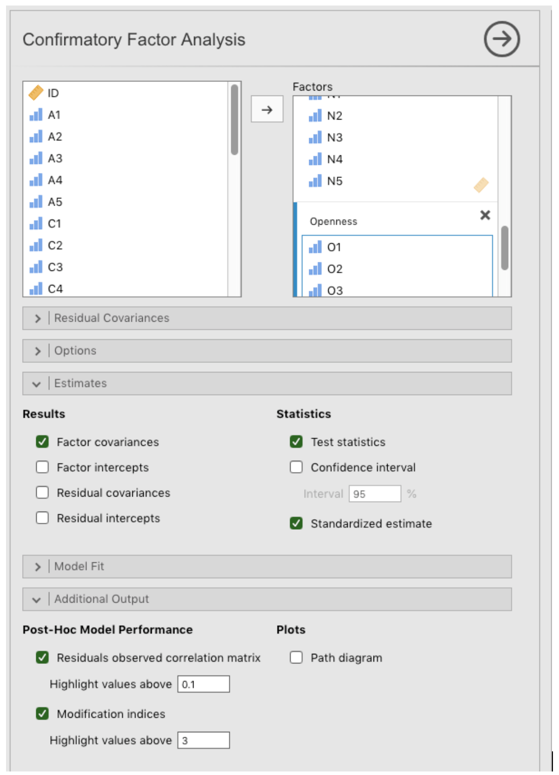
Fig. 192 Options panel with the settings for conducting a Confirmatory Factor Analysis (CFA) in jamovi
Once we have set up the analysis we can turn our attention to the jamovi results window and see what’s what. The first thing to look at is model fit (Fig. 193) as this tells us how good a fit our model is to the observed data. NB in our model only the pre-specified covariances are estimated, including the factor correlations by default. Everything else is set to zero.
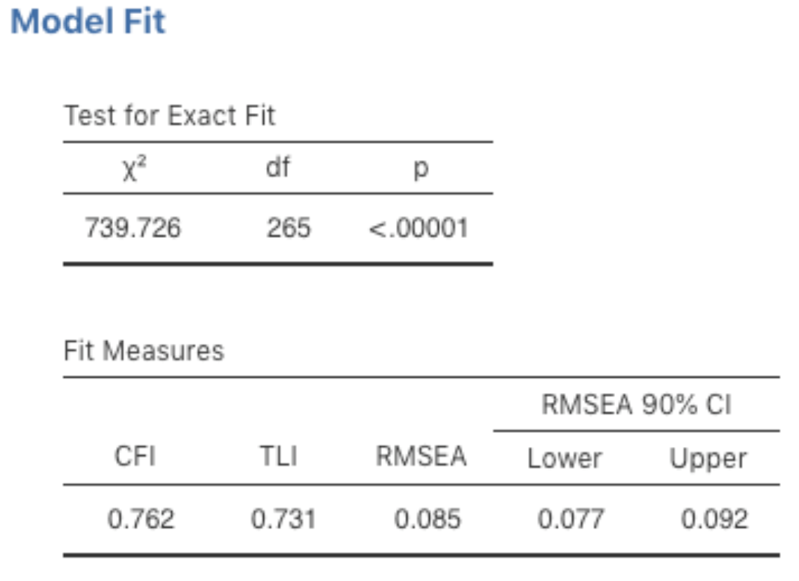
Fig. 193 Table with Model Fit results for the specified CFA model in jamovi
There are several ways of assessing model fit. The first is a χ²-statistic that, if small, indicates that the model is a good fit to the data. However, the χ²-statistic used for assessing model fit is pretty sensitive to sample size, meaning that with a large sample a good enough fit between the model and the data almost always produces a large and significant (p < 0.05) χ²-value.
So, we need some other ways of assessing model fit. jamovi provides several by default. These are the Comparative Fit Index (CFI), the Tucker Lewis Index (TLI) and the Root Mean Square Error of Approximation (RMSEA) together with the 90% confidence interval for the RMSEA. Some useful rules of thumb are that a satisfactory fit is indicated by CFI > 0.9, TLI > 0.9, and RMSEA of about 0.05 to 0.08. A good fit is CFI > 0.95, TLI > 0.95, and RMSEA and upper CI for RMSEA < 0.05.
So, looking at Fig. 193, we can see that the χ²-value is large and highly significant. Our sample size is not too large, so this possibly indicates a poor fit. The CFI is 0.762 and the TLI is 0.731, indicating poor fit between the model and the data. The RMSEA is 0.085 with a 90% confidence interval from 0.077 to 0.092, again this does not indicate a good fit.
Pretty disappointing, huh? But perhaps not too surprising given that in the earlier EFA, when we ran with a similar data set (section Exploratory Factor Analysis), only around half of the variance in the data was accounted for by the five factor model.
Let’s go on to look at the factor loadings and the factor covariance estimates,
shown in Fig. 194 and Fig. 195. The Z-statistic and
p-value for each of these parameters indicates they make a reasonable
contribution to the model (i.e. they are not zero) so there doesn’t appear to
be any reason to remove any of the specified variable-factor paths, or
factor-factor correlations from the model. Often the standardized estimates are
easier to interpret, and these can be specified under the Estimates option.
These tables can usefully be incorporated into a written report or scientific
article.
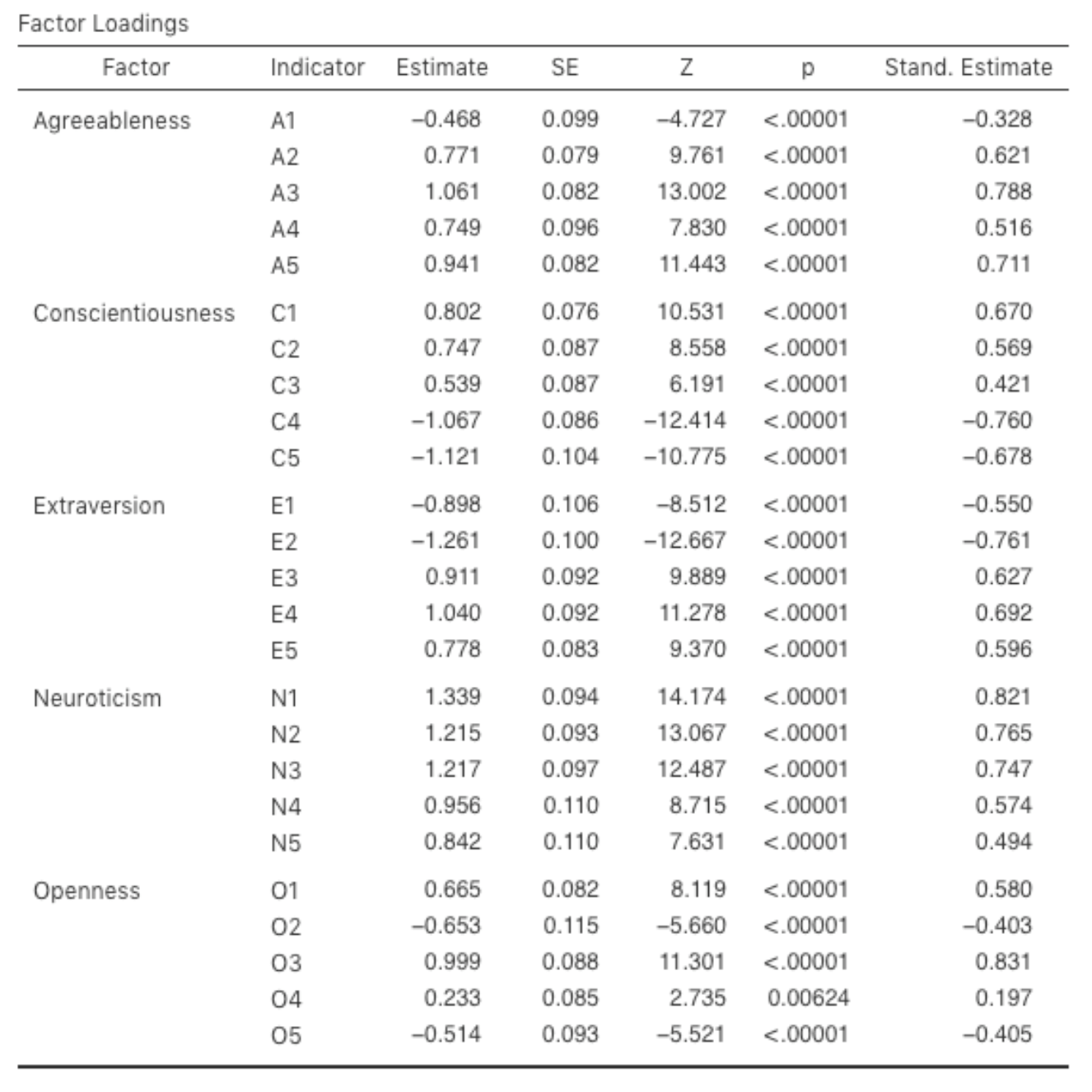
Fig. 194 Table with Factor Loadings for the specified CFA model in jamovi
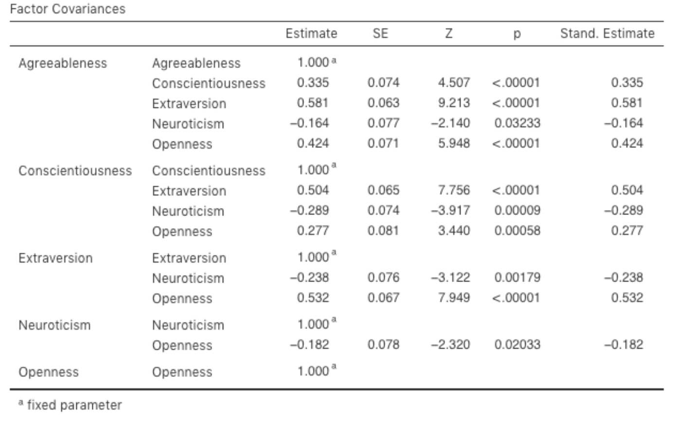
Fig. 195 Table with Factor Covariances for the specified CFA model in jamovi
How could we improve the model? One option is to go back a few stages and think
again about the items / measures we are using and how they might be improved or
changed. Another option is to make some post-hoc tweaks to the model to
improve the fit. One way of doing this is to use Modification indices,
specified as an Additional Output option in jamovi (see Fig. 196).
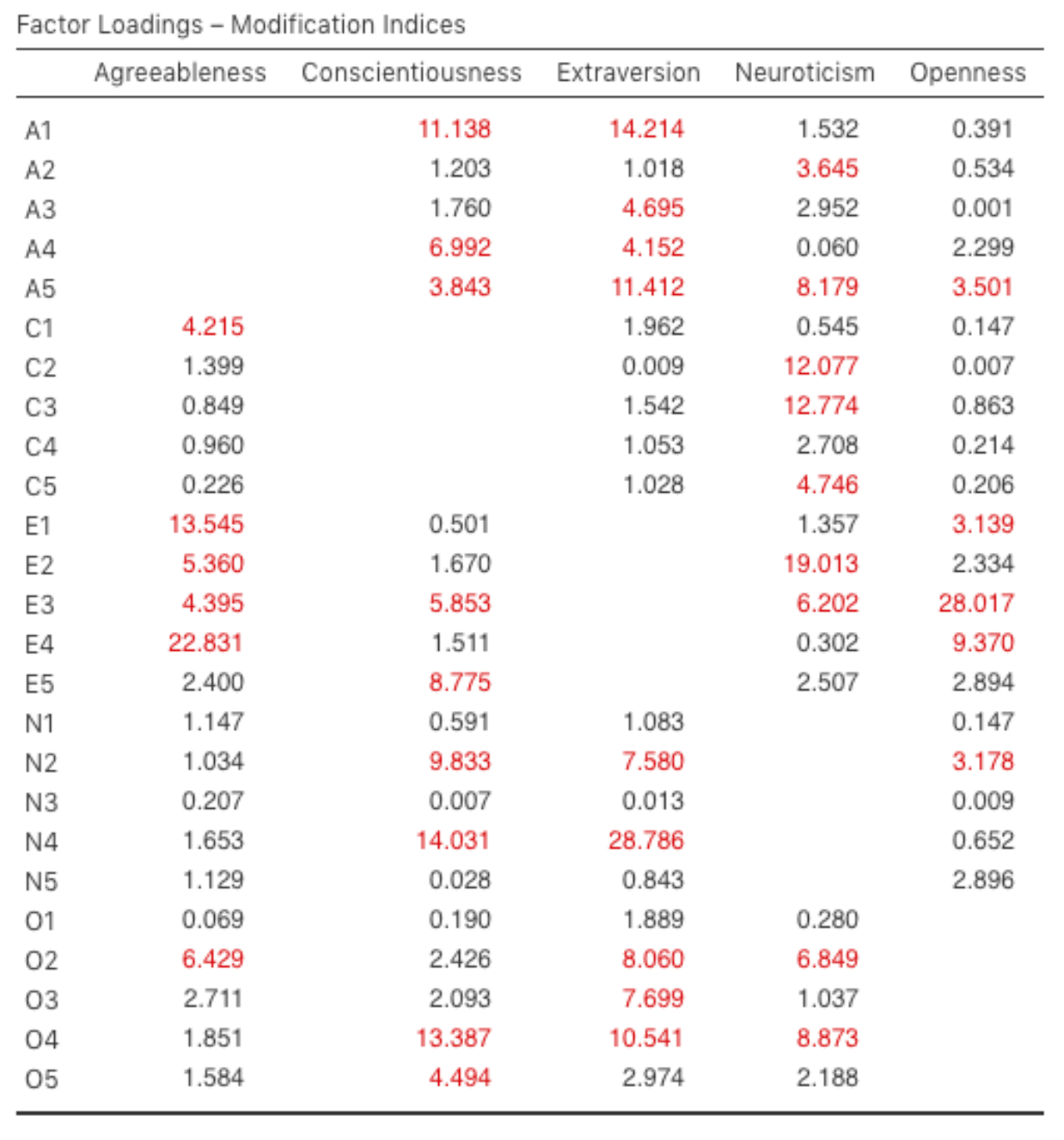
Fig. 196 Table with Factor Loadings Modification Indices for the specified CFA
model in jamovi
What we are looking for is the highest modification index (MI) value. We would
then judge whether it makes sense to add that additional term into the model,
using a post-hoc rationalisation. For example, we can see in
Fig. 196 that the largest MI for the factor loadings that are not
already in the model is a value of 28.786 for the loading of N4 (“Often
feel blue”) onto the latent factor Extraversion. This indicates that if we add
this path into the model then the χ²-value will reduce by around the same amount.
But in our model adding this path arguably doesn’t really make any theoretical
or methodological sense, so it’s not a good idea (unless you can come up with
a persuasive argument that “Often feel blue” measures both Neuroticism and
Extraversion). I can’t think of a good reason. But, for the sake of argument,
let’s pretend it does make some sense and add this path into the model. Go
back to the CFA analysis window (see Fig. 192) and add N4 into
the Extraversion factor. The results of the CFA will now change (not shown);
the χ²-value has come down to around 709 (a drop of around 30, roughly
similar to the size of the MI) and the other fit indices have also improved,
though only a bit. But it’s not enough: it’s still not a good fitting model.
If you do find yourself adding new parameters to a model using the MI values then always re-check the MI tables after each new addition, as the MIs are refreshed each time.
There is also a Table of Residual Covariances Modification Indices produced
by jamovi (Fig. 197). In other words, a table showing which correlated
errors, if added to the model, would improve the model fit the most. It’s a
good idea to look across both MI tables at the same time, spot the largest MI,
think about whether the addition of the suggested parameter can be reasonably
justified and, if it can, add it to the model. And then you can start again
looking for the biggest MI in the re-calculated results.
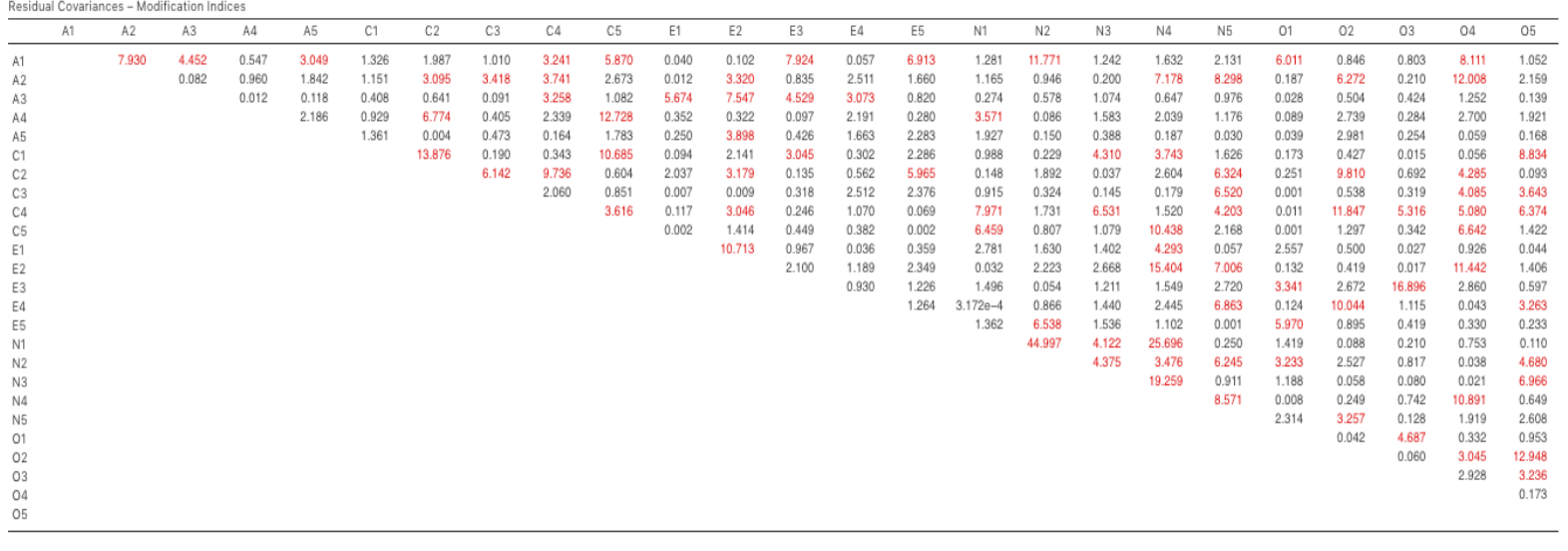
Fig. 197 Table with Residual Covariances Modification Indices for the specified
CFA model in jamovi
You can keep going this way for as long as you like, adding parameters to the model based on the largest MI, and eventually you will achieve a satisfactory fit. But there will also be a strong possibility that in doing this you will have created a monster! A model that is ugly and deformed and doesn’t have any theoretical sense or purity. In other words, be very careful!
So far, we have checked out the factor structure obtained in the EFA using a second sample and CFA. Unfortunately, we didn’t find that the factor structure from the EFA was confirmed in the CFA, so it’s back to the drawing board as far as the development of this personality scale goes.
Whereas there are sometimes good reasons for allowing residuals to covary (or correlate), there were no such reasons to “optimize” the CFA for the model that we defined by including additional factor loadings or residual covariances using modification indices. Nevertheless, let’s discuss how to report the results of a CFA (with a more fitted model).
Reporting a CFA
There is not a formal standard way to write up a CFA, and examples tend to vary by discipline and researcher. That said, there are some fairly standard pieces of information to include in your write-up:
- A theoretical and empirical justification for the hypothesized model.
- A complete description of how the model was specified (e.g. the indicator variables for each latent factor, covariances between latent variables, and any correlations between error terms). A path diagram, like the one in Fig. 193 would be good to include.
- A description of the sample (e.g. demographic information, sample size, sampling method).
- A description of the type of data used (e.g., nominal
 , continuous
) and descriptive statistics.
, continuous
) and descriptive statistics. - Tests of assumptions and estimation method used.
- A description of missing data and how the missing data were handled.
- The software and version used to fit the model.
- Measures, and the criteria used, to judge model fit.
- Any alterations made to the original model based on model fit or modification indices.
- All parameter estimates (i.e., loadings, error variances, latent (co)variances) and their standard errors, probably in a table.
| [1] | As an aside, given that we had a pretty firm idea from our initial “putative” factors, we could just have gone straight to CFA and skipped the EFA step. Whether you use EFA and then go on to CFA, or go straight to CFA, is a matter of judgement and how confident you are initially that you have the model about right (in terms of number of factors and variables). Earlier on in the development of scales, or the identification of underlying latent constructs, researchers tend to use EFA. Later on, as they get closer to a final scale, or if they want to check an established scale in a new sample, then CFA is a good option. |