Section author: Danielle J. Navarro and David R. Foxcroft
Principal Component Analysis
In the previous section we saw that EFA works to identify underlying latent factors. And, as we saw, in one scenario the smaller number of latent factors can be used in further statistical analysis using some sort of combined factor scores.
In this way EFA is being used as a “data reduction” technique. Another type of data reduction technique, sometimes seen as part of the EFA family, is principal component analysis (PCA). However, PCA does not identify underlying latent factors. Instead it creates a linear composite score from a larger set of measured variables.
PCA simply produces a mathematical transformation to the original data with no assumptions about how the variables co-vary. The aim of PCA is to calculate a few linear combinations (components) of the original variables that can be used to summarize the observed data set without losing much information. However, if identification of underlying structure is a goal of the analysis, then EFA is to be preferred. And, as we saw, EFA produces factor scores that can be used for data reduction purposes just like principal component scores (Fabrigar et al., 1999).
PCA has been popular in Psychology for a number of reasons, and therefore it’s
worth covering, although nowadays EFA is just as easy to do given the power of
desktop computers and can be less susceptible to bias than PCA, especially with
a small number of factors and variables. We’ll use the same bfi_sample
dataset as before. Much of the procedure is similar to EFA, so although there
are some conceptual differences, practically the steps are the same,[1] and
with large samples and a sufficient number of factors and variables, the
results from PCA and EFA should be fairly similar.
Performing PCA in jamovi
Once you have loaded up the bfi_sample data set, select Factor →
Principal Component Analysis from the Analyses tab to open
the options panel where you can determine the settings for the PCA
(Fig. 185). Then select the 25 personality questions and transfer
them into the Variables box. Check appropriate options, including
Assumption Checks, but also Rotation under Method, Number of
Factors to extract, and the Additional Output options (see
Fig. 185 for suggested options for this PCA, and please note that
Rotation under Method and Number of Factors extracted is typically
adjusted during the analysis to find the best result, as described below).
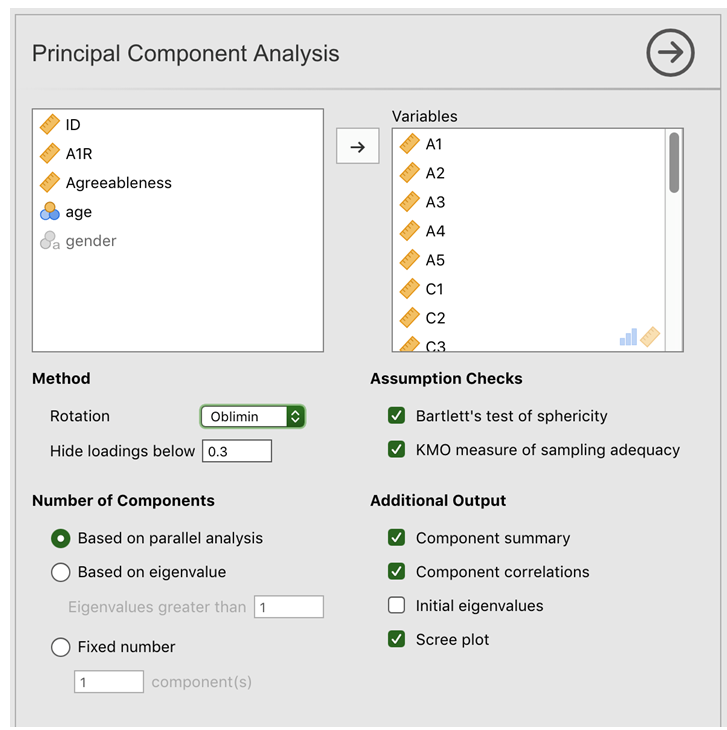
Fig. 185 Options panel with the settings for conducting a Principal Component Analysis (PCA) in jamovi
First, checking the assumptions (see Fig. 186), you can see that (1) Bartlett’s test of sphericity is significant, so this assumption is satisfied; and (2) the KMO measure of sampling adequacy (MSA) is 0.81 overall, suggesting very good sampling adequacy. No problems here then!
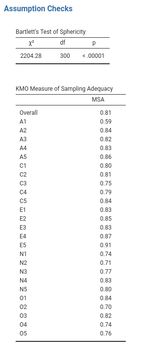
Fig. 186 Assumption checks for the personality item data when using a PCA in jamovi
The next thing to check is how many components to use (or “extract” from the data). As with EFA, three different approaches are available:
- One convention is to choose all components with Eigen values greater than 1. This would give us two components with our data.
- Examination of the scree plot, as in Fig. 187, lets you identify the “point of inflection”. This is the point at which the slope of the scree curve clearly levels off, below the “elbow”. Again, this would give us two components as the levelling off clearly occurs after the second component.
- Using a parallel analysis technique, the obtained Eigen values are compared to those that would be obtained from random data. The number of components extracted is the number with Eigen values greater than what would be found with random data.
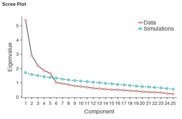
Fig. 187 Scree plot of the personality item data when conducting a PCA in jamovi, showing the levelling off point, the “elbow”, after component 5
The third approach is a good one according to Fabrigar et al. (1999), although in practice researchers tend to look at all three and then make a judgement about the number of components that are most easily or helpfully interpreted. This can be understood as the “meaningfulness criterion”, and researchers will typically examine, in addition to the solution from one of the approaches above, solutions with one or two more or fewer components. They then adopt the solution which makes the most sense to them.
At the same time, we should also consider the best way to rotate the final
solution. Again, as with EFA, there are two main approaches to rotation:
orthogonal (e.g. Varimax) rotation forces the selected components to be
uncorrelated; whereas oblique (e.g. Oblimin) rotation allows the selected
components to be correlated. Dimensions of interest to psychologists and
behavioural scientists are not often dimensions we would expect to be
orthogonal, so oblique solutions are arguably more sensible. Practically, if in
an oblique rotation the components are found to be substantially correlated
(i.e. > 0.3) then this would confirm our intuition to prefer oblique rotation.
If the components are, in fact, correlated, then an oblique rotation will
produce a better estimate of the true components and a better simple structure
than will an orthogonal rotation. And, if the oblique rotation indicates that
the components have close to zero correlations between one another, then the
researcher can go ahead and conduct an orthogonal rotation (which should then
give about the same solution as the oblique rotation). In Fig. 188
we see that none of the correlations is > 0.3 so it is appropriate to switch to
orthogonal (Varimax) rotation.
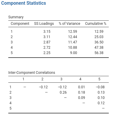
Fig. 188 Component summary statistics and correlations for a five component solution when conducting a PCA with the personality item data in jamovi
In Fig. 188 we also have the proportion of overall variance in the data that is accounted for by the two components. Components one and two account for just over 12% of the variance each. Taken together, the five component solution accounts for just over half of the variance (56%) in the observed data. Be aware that in every PCA you could potentially have the same number of components as observed variables, but every additional component you include will add a smaller amount of explained variance. If the first few components explain a good amount of the variance in the original 25 variables, then those components are clearly a useful, simpler substitute for all 25 variables. You can drop the rest without losing too much of the original variability. But if it takes 18 components to explain most of the variance in those 25 variables, you might as well just use the original 25.
Fig. 189 shows the component loadings. That’s is, how the 25 different personality items load onto each of the selected components. We have hidden loadings less than 0.4 (set in the options shown in Fig. 185) as we were interested in items with a substantive loading and setting the threshold at the higher 0.4 value also provided a cleaner, clearer solution.
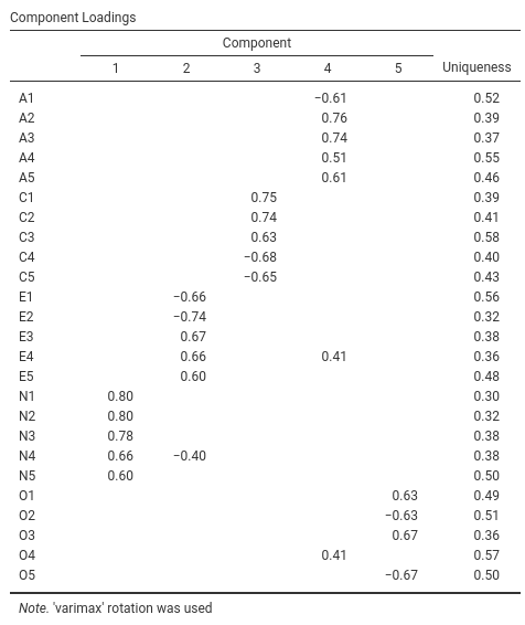
Fig. 189 Component loadings for a five component solution when conducting a PCA with the personality item data in jamovi
For components 1, 2, 3 and 4 the pattern of component loadings closely matches
the putative factors specified in Table 18. And component 5 is pretty
close, with four of the five observed variables that putatively measure
“Openness” loading pretty well onto the component. Variable O4 doesn’t
quite seem to fit though, as the component solution in Fig. 189
suggests that it loads onto component 4 (albeit with a relatively low loading)
but not substantively onto component 5.
We can also see in Fig. 185 the Uniqueness of each variable.
Uniqueness is the proportion of variance that is “unique” to the variable and
not explained by the components. For example, 52% of the variance in A1 is
not explained by the components in the five component solution. In contrast,
N1 has relatively low variance not accounted for by the component solution
(30%). Note that the greater the Uniqueness, the lower the relevance or
contribution of the variable in the component model.
Hopefully, this has given you a good first idea about how to undertake PCA in jamovi, and how it is conceptually different but practically fairly similar (given the right data) to EFA.
You can go on to create and save component scores in much the same way as in
EFA. However, if you take the option to create an optimally-weighted component
score index then the commands and syntax in the jamovi Rj editor are a
little different. See Fig. 190.
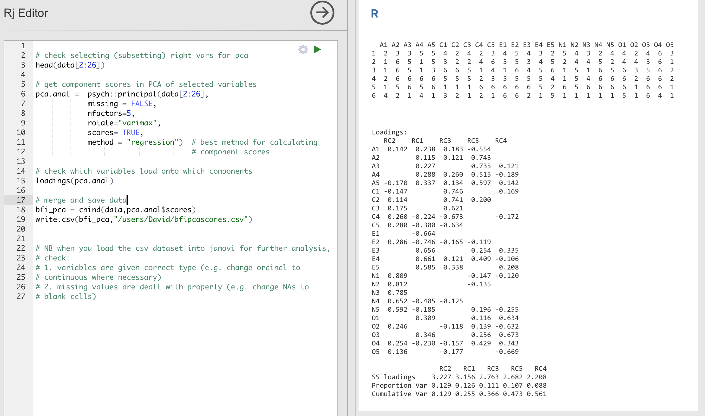
Fig. 190 Rj editor commands for creating optimally weighted component scores for
the five component solution when conducting a PCA with the personality item
data in jamovi
| [1] | …and that means there is a fair bit of repetition in the PCA steps set out in the next section. Sorry about that, but hopefully it is not too bad! |