Section author: Danielle J. Navarro and David R. Foxcroft
Exploratory Factor Analysis
Exploratory Factor Analysis (EFA) is a statistical technique for revealing any hidden latent factors that can be inferred from our observed data. This technique calculates to what extent a set of measured variables, for example V1, V2, V3, V4, and V5, can be represented as measures of an underlying latent factor. This latent factor cannot be measured through just one observed variable but instead is manifested in the relationships it causes in a set of observed variables.
In Fig. 174 each observed variable V is “caused” to some extent by the underlying latent factor (F), depicted by the coefficients b1 to b5 (also called factor loadings). Each observed variable also has an associated error term, e1 to e5. Each error term is the variance in the associated observed variable, Vi, that is unexplained by the underlying latent factor.
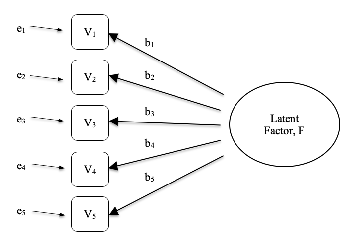
Fig. 174 Latent factor underlying the relationship between several observed variables
In Psychology, latent factors represent psychological phenomena or constructs that are difficult to directly observe or measure. For example, personality, or intelligence, or thinking style. In the example in Fig. 174, we may have asked people five specific questions about their behaviour or attitudes, and from that we are able to get a picture about a personality construct called, for example, extraversion. A different set of specific questions may give us a picture about an individual’s introversion, or their conscientiousness.
Here’s another example: we may not be able to directly measure statistics anxiety, but we can measure whether statistics anxiety is high or low with a set of questions in a questionnaire. For example, “Q1: Doing the assignment for a statistics course”, “Q2: Trying to understand the statistics described in a journal article”, and “Q3: Asking the lecturer for help in understanding something from the course”, etc., each rated from low anxiety to high anxiety. People with high statistics anxiety will tend to give similarly high responses on these observed variables because of their high statistics anxiety. Likewise, people with low statistics anxiety will give similar low responses to these variables because of their low statistics anxiety.
In exploratory factor analysis (EFA), we are essentially exploring the correlations between observed variables to uncover any interesting, important underlying (latent) factors that are identified when observed variables co-vary. We can use statistical software to estimate any latent factors and to identify which of our variables have a high loading[1] (e.g. loading > 0.5) on each factor, suggesting they are a useful measure, or indicator, of the latent factor. Part of this process includes a step called rotation, which to be honest is a pretty weird idea but luckily we don’t have to worry about understanding it; we just need to know that it is helpful because it makes the pattern of loadings on different factors much clearer. As such, rotation helps with seeing more clearly which variables are linked substantively to each factor. We also need to decide how many factors are reasonable given our data, and helpful in this regard is something called Eigen values. We’ll come back to this in a moment, after we have covered some of the main assumptions of EFA.
Checking assumptions
There are a couple of assumptions that need to be checked as part of the analysis. The first assumption is sphericity, which essentially checks that the variables in your dataset are correlated with each other to the extent that they can potentially be summarised with a smaller set of factors. Bartlett’s test for sphericity checks whether the observed correlation matrix diverges significantly from a zero (or null) correlation matrix. So, if Bartlett’s test is significant (p < 0.05), this indicates that the observed correlation matrix is significantly divergent from the null, and is therefore suitable for EFA.
The second assumption is sampling adequacy and is checked using the Kaiser-Meyer-Olkin (KMO) Measure of Sampling Adequacy (MSA). The KMO index is a measure of the proportion of variance among observed variables that might be common variance. Using partial correlations, it checks for factors that load just two items. We seldom, if ever, want EFA producing a lot of factors loading just two items each. KMO is about sampling adequacy because partial correlations are typically seen with inadequate samples. If the KMO index is high (≈ 1), the EFA is efficient whereas if KMO is low (≈ 0), the EFA is not relevant. KMO values smaller than 0.5 indicates that EFA is not suitable and a KMO value of 0.6 should be present before EFA is considered suitable. Values between 0.5 and 0.7 are considered adequate, values between 0.7 and 0.9 are good and values between 0.9 and 1.0 are excellent.
What is EFA good for?
If the EFA has provided a good solution (i.e. factor model), then we need to decide what to do with our shiny new factors. Researchers often use EFA during psychometric scale development. They will develop a pool of questionnaire items that they think relate to one or more psychological constructs, use EFA to see which items “go together” as latent factors, and then they will assess whether some items should be removed because they don’t usefully or distinctly measure one of the latent factors.
In line with this approach, another consequence of EFA is to combine the variables that load onto distinct factors into a factor score, sometimes known as a scale score. There are two options for combining variables into a scale score:
- Create a new variable with a score weighted by the factor loadings for each item that contributes to the factor.
- Create a new variable based on each item that contributes to the factor, but weighting them equally.
In the first option each item’s contribution to the combined score depends on how strongly it relates to the factor. In the second option we typically just average across all the items that contribute substantively to a factor to create the combined scale score variable. Which to choose is a matter of preference, though a disadvantage with the first option is that loadings can vary quite a bit from sample to sample, and in behavioural and health sciences we are often interested in developing and using composite questionnaire scale scores across different studies and different samples. In which case it is reasonable to use a composite measure that is based on the substantive items contributing equally rather than weighting by sample specific loadings from a different sample. In any case, understanding a combined variable measure as an average of items is simpler and more intuitive than using a sample specific optimally-weighted combination.
A more advanced statistical technique, one which is beyond the scope of this book, undertakes regression modelling where latent factors are used in prediction models of other latent factors. This is called “structural equation modelling” and there are specific software programmes and R packages dedicated to this approach. But let’s not get ahead of ourselves; what we should really focus on now is how to do an EFA in jamovi.
EFA in jamovi
First, we need some data. Twenty-five personality self-report items (see Table 18) taken from the International Personality Item Pool (https://ipip.ori.org) were included as part of the Synthetic Aperture Personality Assessment (SAPA) web-based personality assessment (https://sapa-project.org) project. The 25 items are short phrases that one should respond to by indicating how accurately the statement describes one’s typical behaviour or attitudes. The items are organized by five putative factors: Agreeableness, Conscientiousness, Extraversion, Neuroticism, and Openness.
| Name | Question / Item | |
|---|---|---|
| A1 | R | Am indifferent to the feelings of others. |
| A2 | Inquire about others’ well-being. | |
| A3 | Know how to comfort others. | |
| A4 | Love children. | |
| A5 | Make people feel at ease. | |
| C1 | Am exacting in my work. | |
| C2 | Continue until everything is perfect. | |
| C3 | Do things according to a plan. | |
| C4 | R | Do things in a half-way manner. |
| C5 | R | Waste my time. |
| E1 | R | Don’t talk a lot. |
| E2 | R | Find it difficult to approach others. |
| E3 | Know how to captivate people. | |
| E4 | Make friends easily. | |
| E5 | Take charge. | |
| N1 | Get angry easily. | |
| N2 | Get irritated easily. | |
| N3 | Have frequent mood swings. | |
| N4 | Often feel blue. | |
| N5 | Panic easily. | |
| O1 | Am full of ideas. | |
| O2 | R | Avoid difficult reading material. |
| O3 | Carry the conversation to a higher level. | |
| O4 | Spend time reflecting on things. | |
| O5 | R | Will not probe deeply into a subject. |
The item data were collected using a 6-point response scale:
- Very Inaccurate
- Moderately Inaccurate
- Slightly Inaccurate
- Slightly Accurate
- Moderately Accurate
- Very Accurate.
A sample of N = 250 responses is contained in the bfi_sample data set. In
addition to the items, there are three further columns in the data set: ID
(the respondent ID, a five digit number) as well as the age (age) and the
gender (gender) of the respondent.
As researchers, we are interested in exploring the data to see whether there
are some underlying latent factors that are measured reasonably well by the 25
observed variables in the bfi_sample data set. Open it up and check that the
25 variables are coded as continuous variables  (technically they
are ordinal
(technically they
are ordinal  though for EFA in jamovi it mostly doesn’t matter, except
if you decide to calculate weighted factor scores in which case continuous
variables are needed). To perform an EFA in jamovi:
though for EFA in jamovi it mostly doesn’t matter, except
if you decide to calculate weighted factor scores in which case continuous
variables are needed). To perform an EFA in jamovi:
- Select
Factor→Exploratory Factor Analysisfrom theAnalysestab to open the options panel where you can determine the settings for the EFA (Fig. 175). - Select the 25 personality questions and transfer them into the
Variablesbox. - Check appropriate options, including
Assumption Checks, but alsoRotationunderMethod,Number of Factorsto extract, andAdditional Outputoptions (see Fig. 175 for suggested options for this illustrative EFA, and please note that theRotationunderMethodandNumber of Factorsextracted is typically adjusted by the researcher during the analysis to find the best result, as described below).
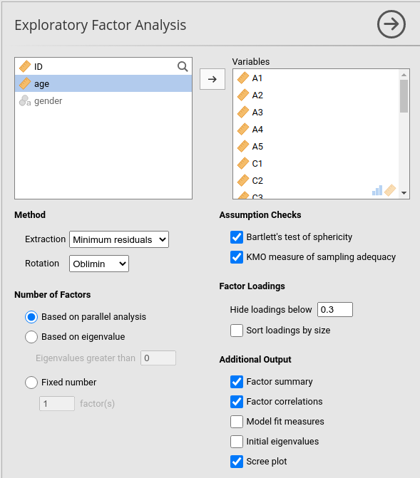
Fig. 175 Options panel with the settings for conducting an Exploratory Factor Analysis (EFA) in jamovi
First, check the assumptions (Fig. 176). You can see that (1) Bartlett’s test of sphericity is significant, so this assumption is satisfied; and (2) the KMO measure of sampling adequacy (MSA) is 0.81 overall, suggesting good sampling adequacy. No problems here then!
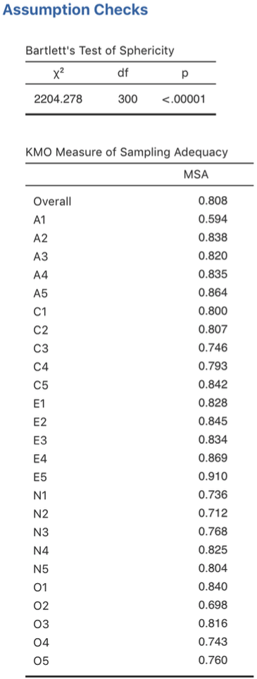
Fig. 176 jamovi EFA assumption checks for the personality questionnaire data
The next thing to check is how many factors to use (or “extract” from the data). Three different approaches are available:
- One convention is to choose all components with Eigen values greater than 1.[2] This would give us four factors with our data (try it and see).
- Examination of the scree plot, as in Fig. 177, lets you identify the “point of inflection”. This is the point at which the slope of the scree curve clearly levels off, below the “elbow”. This would give us five factors with our data. Interpreting scree plots is a bit of an art: in Fig. 177 there is a noticeable step from 5 to 6 factors, but in other scree plots you look at it will not be so clear cut.
- Using a parallel analysis technique, the obtained Eigen values are compared to those that would be obtained from random data. The number of factors extracted is the number with Eigen values greater than what would be found with random data.
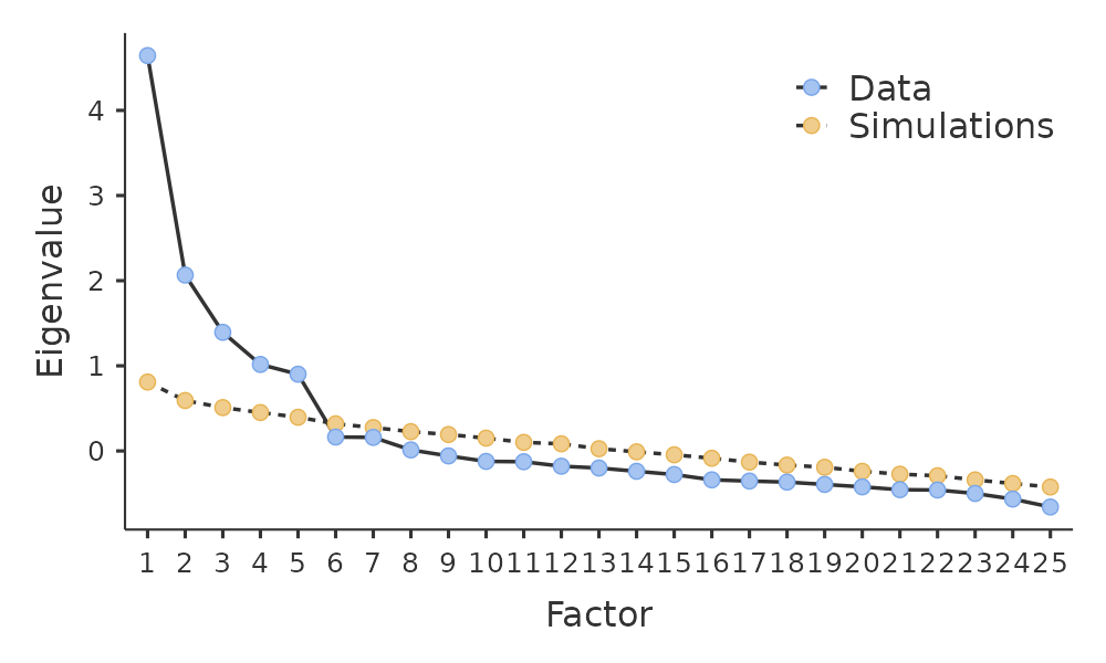
Fig. 177 Scree plot of the personality data in the EFA in jamovi, showing a noticeable inflection and levelling off after point 5 (the “elbow”)
The third approach is a good one according to Fabrigar et al. (1999), although in practice researchers tend to look at all three and then make a judgement about the number of factors that are most easily or helpfully interpreted. This can be understood as the “meaningfulness criterion”, and researchers will typically examine, in addition to the solution from one of the approaches above, solutions with one or two more or fewer factors. They then adopt the solution which makes the most sense to them.
At the same time, we should also consider the best way to rotate the final
solution. There are two main approaches to rotation: orthogonal (e.g.
Varimax) rotation forces the selected factors to be uncorrelated, whereas
oblique (e.g. Oblimin) rotation allows the selected factors to be
correlated. Dimensions of interest to psychologists and behavioural scientists
are not often dimensions we would expect to be orthogonal, so oblique solutions
are arguably more sensible.[3]
Practically, if in an oblique rotation the factors are found to be substantially correlated (positive or negative, and > 0.3), as in Fig. 178 where a correlation between two of the extracted factors is 0.31, then this would confirm our intuition to prefer oblique rotation. If the factors are, in fact, correlated, then an oblique rotation will produce a better estimate of the true factors and a better simple structure than will an orthogonal rotation. And, if the oblique rotation indicates that the factors have close to zero correlations between one another, then the researcher can go ahead and conduct an orthogonal rotation (which should then give about the same solution as the oblique rotation).
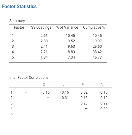
Fig. 178 Factor summary statistics and correlations for a five factor solution in the EFA conducted in jamovi
On checking the correlation between the extracted factors at least one
correlation was greater than 0.3 (Fig. 178), so an oblique
(Oblimin) rotation of the five extracted factors is preferred. We can also
see in Fig. 178 that the proportion of overall variance in the data
that is accounted for by the five factors is 46%. Factor one accounts for
around 10% of the variance, factors two to four around 9% each, and factor five
just over 7%. This isn’t great; it would have been better if the overall
solution accounted for a more substantive proportion of the variance in our
data.
Be aware that in every EFA you could potentially have the same number of factors as observed variables, but every additional factor you include will add a smaller amount of explained variance. If the first few factors explain a good amount of the variance in the original 25 variables, then those factors are clearly a useful, simpler substitute for the 25 variables. You can drop the rest without losing too much of the original variability. But if it takes 18 factors (for example) to explain most of the variance in those 25 variables, you might as well just use the original 25.
Fig. 179 shows the factor loadings. That is, how the 25 different personality items load onto each of the five selected factors. We have hidden loadings less than 0.3 (set in the options shown in Fig. 175).
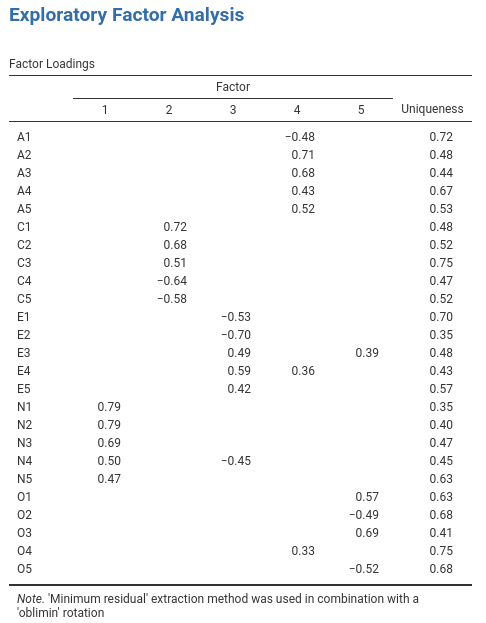
Fig. 179 Factor loadings for a five factor solution in the EFA conducted in jamovi
For factors 1, 2, 3 and 4 the pattern of factor loadings closely matches the
putative factors specified in Table 18. Phew! And factor 5 is pretty
close, with four of the five observed variables that putatively measure
“Openness” loading pretty well onto the factor. Variable O4 doesn’t quite
seem to fit though, as the factor solution in Fig. 179 suggests that
it loads onto factor 4 (albeit with a relatively low loading) but not
substantively onto factor 5.
The other thing to note is that those variables that were denoted as “R:
reverse coding” in Table 18 are those that have negative factor
loadings. Take a look at the items A1 (“Am indifferent to the feelings of
others”) and A2 (“Inquire about others’ well-being”). We can see that a
high score on A1 indicates low Agreeableness, whereas a high score on
A2 (and all the other A-variables for that matter) indicates high
Agreeableness. Therefore A1 will be negatively correlated with the other
A-variables, and this is why it has a negative factor loading, as shown
in Fig. 179.
We can also see in Fig. 179 the Uniqueness of each variable.
Uniqueness is the proportion of variance that is “unique” to the variable and
not explained by the factors.[4] For example, 72% of the variance in A1
is not explained by the factors in the five factor solution. In contrast,
N1 has relatively low variance not accounted for by the factor solution
(35%). Note that the greater the Uniqueness, the lower the relevance or
contribution of the variable in the factor model.
To be honest, it’s unusual to get such a neat solution in EFA. It’s typically quite a bit more messy than this, and often interpreting the meaning of the factors is more challenging. It’s not often that you have such a clearly delineated item pool. More often you will have a whole heap of observed variables that you think may be indicators of a few underlying latent factors, but you don’t have such a strong sense of which variables are going to go where!
So, we seem to have a pretty good five factor solution, albeit accounting for
a relatively low overall proportion of the observed variance. Let’s assume we
are happy with this solution and want to use our factors in further analysis.
The straightforward option is to calculate an overall (average) score for each
factor by adding together the score for each variable that loads substantively
onto the factor and then dividing by the number of variables. For each person
in our dataset that would mean, for example for the Agreeableness factor,
adding together A1 + A2 + A3 + A4 + A5, and then dividing by 5.[5]
In essence, this means that the factor score we have calculated is based on
equally weighted scores from each of the included variables. We can do this in
jamovi in two steps:
- Recode
A1intoA1Rby reverse scoring the values in the variable (i.e. 6 = 1; 5 = 2; 4 = 3; 3 = 4; 2 = 5; 1 = 6) using the jamovi transform variable command (see Fig. 180). - Compute a new variable, called
Agreeableness, by calculating the mean ofA1R,A2,A3,A4andA5. Do this using the jamoviComputecommand to create a new variable (see Fig. 181).
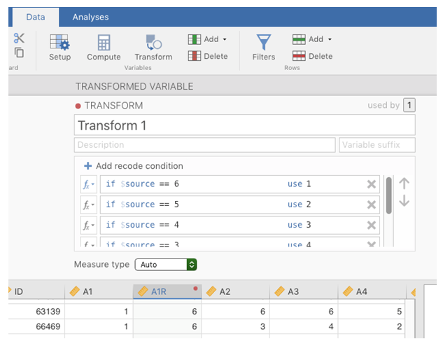
Fig. 180 Recode variable using the Transform command in jamovi
Fig. 181 Compute new scale score variable using a Computed variable in jamovi
Another option is to create an optimally-weighted factor score index. We can
use the jamovi Rj editor to do this in R.[6] Again, there are two
steps:
- Use the
Rjeditor to run the EFA inRto the same specification as the one in jamovi (i.e., five factors and Oblimin rotation) and compute optimally weighted factor scores. Save the new dataset, with the factor scores, to a file (see Fig. 182). - Open up the new file in jamovi (see Fig. 183) and check that variable types have been set correctly. Label the new factor score variables corresponding to the relevant factor names or definitions (NB: it is possible that the factors will not be in the expected order, so make sure you check).
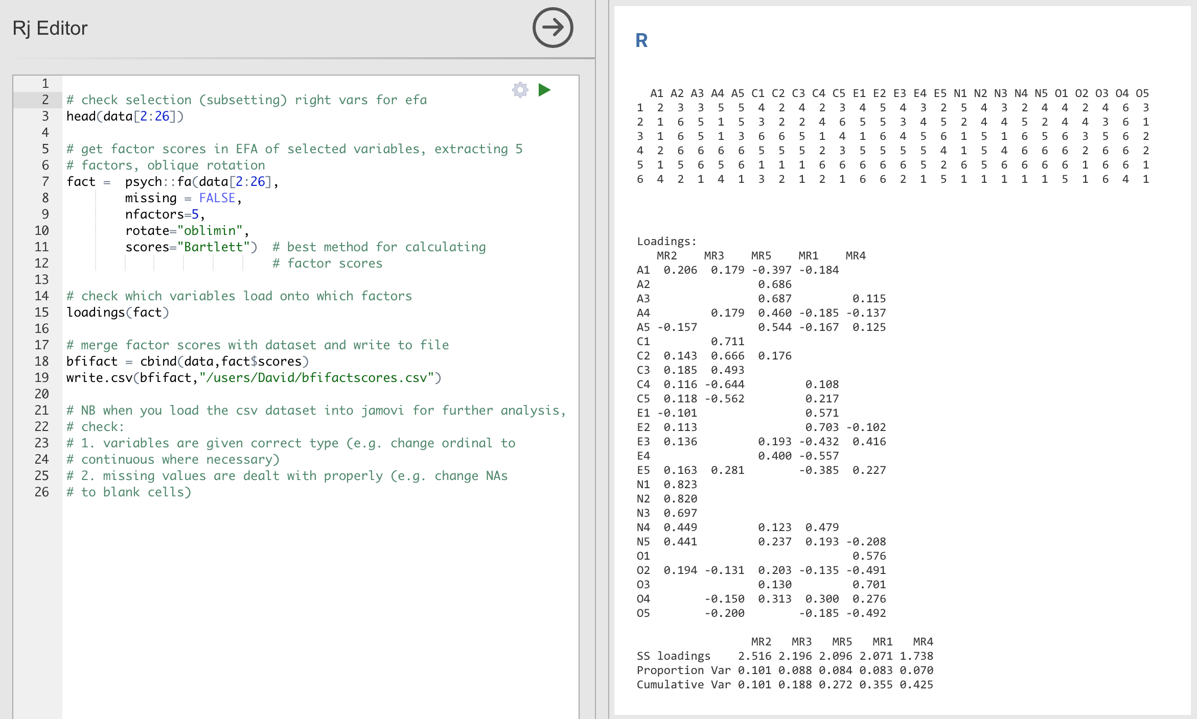
Fig. 182 Rj editor commands for creating optimally weighted factor scores for
the five factor solution
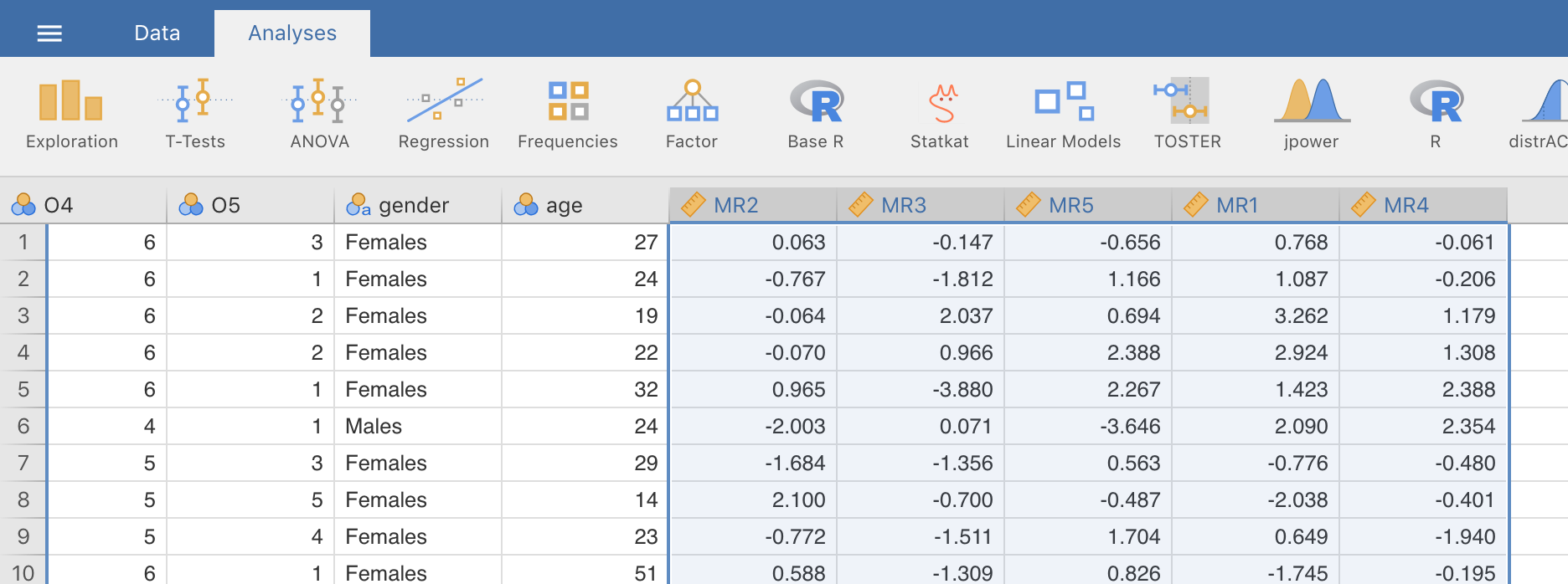
Fig. 183 Newly created data file bfifactscores.csv created in the Rj editor,
and containing the five factor score variables. Note that each of the new
factor score variables is labelled corresponding to the order that the
factors are listed in the factor loadings table.
Now you can go ahead and undertake further analyses, using either the factor-
based scores (a mean scale score approach) or using the optimally-weighted
factor scores calculated via the Rj editor. Your choice! For example, one
thing you might like to do is see whether there are any gender differences in
each of our personality scales. We did this for the Agreeableness score that we
calculated using the factor-based score approach, and although the plot (see
Fig. 184) showed that males were less agreeable than females, this
was not a significant difference (Mann-Whitney U = 5760.5, p = 0.073).
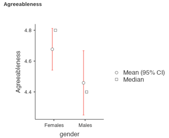
Fig. 184 Comparing differences in Agreeableness factor-based scores between males and females
Writing up an EFA
Hopefully, so far we have given you some sense of EFA and how to undertake EFA in jamovi. So, once you have completed your EFA, how do you write it up? There is not a formal standard way to write up an EFA, and examples tend to vary by discipline and researcher. That said, there are some fairly standard pieces of information to include in your write-up:
- What are the theoretical underpinnings for the area you are studying, and specifically for the constructs that you are interested in uncovering through EFA.
- A description of the sample (e.g. demographic information, sample size, sampling method).
- A description of the type of data used (e.g., nominal
 , continuous
) and descriptive statistics.
, continuous
) and descriptive statistics. - Describe how you went about testing the assumptions for EFA. Details regarding sphericity checks and measures of sampling adequacy should be reported.
- Explain what FA extraction method (e.g. maximum likelihood) was used.
- Explain the criteria and process used for deciding how many factors were extracted in the final solution, and which items were selected. Clearly explain the rationale for key decisions during the EFA process.
- Explain what rotation methods were attempted, the reasons why, and the results.
- Final factor loadings should be reported in the results, in a table. This table should also report the uniqueness (or communality) for each variable (in the final column). Factor loadings should be reported with descriptive labels in addition to item numbers. Correlations between the factors should also be included, either at the bottom of this table, in a separate table.
- Meaningful names for the extracted factors should be provided. You may like to use previously selected factor names, but on examining the actual items and factors you may think a different name is more appropriate.
| [1] | Quite helpfully, factor loadings can be interpreted like standardized regression coefficients |
| [2] | An Eigen value indicates how much of the variance in the observed variables a factor accounts for. A factor with an Eigen value > 1 accounts for more variance than a single observed variable |
| [3] | Oblique rotations provide two factor matrices, one called a structure matrix and one called a pattern matrix. In jamovi just the pattern matrix is shown in the results as this is typically the most useful for interpretation, though some experts suggest that both can be helpful. In a structure matrix coefficients show the relationship between the variable and the factors whilst ignoring the relationship of that factor with all the other factors (i.e. a zero-order correlation). Pattern matrix coefficients show the unique contribution of a factor to a variable whilst controlling for the effects of other factors on that variable (akin to standardized partial regression coefficient). Under orthogonal rotation, structure and pattern coefficients are the same. |
| [4] | Sometimes reported in factor analysis is “communality” which is the amount of variance in a variable that is accounted for by the factor solution. Uniqueness is equal to (1 - communality) |
| [5] | Remembering to first reverse score some variables if necessary. |
| [6] | In the latest versions of jamovi you can now save factor scores directly from within jamovi - it’s an option. But this explanation is helpful as it’s a good insight into using R directly from jamovi. |