Section author: Danielle J. Navarro and David R. Foxcroft
Effect size
The effect size calculation for a factorial ANOVA is pretty similar to those used in One-Way ANOVA (see section Effect size). Specifically, we can use η² (eta-squared) as a simple way to measure how big the overall effect is for any particular term. As before, η² is defined by dividing the sum of squares associated with that term by the total sum of squares. For instance, to determine the size of the main effect of Factor A, we would use the following formula:
As before, this can be interpreted in much the same way as R² in regression.[1] It tells you the proportion of variance in the outcome variable that can be accounted for by the main effect of Factor A. It is therefore a number that ranges from 0 (no effect at all) to 1 (accounts for all of the variability in the outcome). Moreover, the sum of all the η² values, taken across all the terms in the model, will sum to the the total R² for the ANOVA model. If, for instance, the ANOVA model fits perfectly (i.e., there is no within-groups variability at all!), the η² values will sum to 1. Of course, that rarely if ever happens in real life.
However, when doing a factorial ANOVA, there is a second measure of effect size that people like to report, known as partial η². The idea behind partial η² (which is sometimes denoted pη² or η²p) is that, when measuring the effect size for a particular term (say, the main effect of Factor A), you want to deliberately ignore the other effects in the model (e.g., the main effect of Factor B). That is, you would pretend that the effect of all these other terms is zero, and then calculate what the η²-value would have been. This is actually pretty easy to calculate. All you have to do is remove the sum of squares associated with the other terms from the denominator. In other words, if you want the partial η² for the main effect of Factor A, the denominator is just the sum of the SS values for Factor A and the residuals
This will always give you a larger number than η², which the cynic in me suspects accounts for the popularity of partial η². And once again you get a number between 0 and 1, where 0 represents no effect. However, it’s slightly trickier to interpret what a large partial η² value means. In particular, you can’t actually compare the partial η² values across terms! Suppose, for instance, there is no within-groups variability at all: if so, SSR = 0. What that means is that every term has a partial η² value of 1. But that doesn’t mean that all terms in your model are equally important, or indeed that they are equally large. All it mean is that all terms in your model have effect sizes that are large relative to the residual variation. It is not comparable across terms.
To see what I mean by this, it’s useful to see a concrete example. First, let’s have a look at the effect sizes for the original ANOVA without the interaction term, from Fig. 146:
              eta.sq partial.eta.sq
drug           0.71        0.79
therapy        0.10        0.34
Looking at the η² values first, we see that drug accounts for 71% of the
variance (i.e. η² = 0.71) in mood.gain, whereas therapy only accounts
for 10%. This leaves a total of 19% of the variation unaccounted for (i.e., the
residuals constitute 19% of the variation in the outcome). Overall, this
implies that we have a very large effect[2] of drug and a modest effect
of therapy.
Now let’s look at the partial η² values, shown in Fig. 146.
Because the effect of therapy isn’t all that large, controlling for it
doesn’t make much of a difference, so the partial η² for drug doesn’t
increase very much, and we obtain a value of pη² = 0.79). In contrast,
because the effect of drug was very large, controlling for it makes a big
difference, and so when we calculate the partial η² for therapy you can see
that it rises to pη² = 0.34. The question that we have to ask
ourselves is, what do these partial η² values actually mean? The way I
generally interpret the partial η² for the main effect of Factor A is to
interpret it as a statement about a hypothetical experiment in which only
Factor A was being varied. So, even though in this experiment we varied both
A and B, we can easily imagine an experiment in which only Factor A was varied,
and the partial η² statistic tells you how much of the variance in the outcome
variable you would expect to see accounted for in that experiment. However, it
should be noted that this interpretation, like many things associated with main
effects, doesn’t make a lot of sense when there is a large and significant
interaction effect.
Speaking of interaction effects, here’s what we get when we calculate the effect sizes for the model that includes the interaction term, as in Fig. 150. As you can see, the η² values for the main effects don’t change, but the partial η² values do:
               eta.sq partial.eta.sq
drug            0.71        0.84
therapy         0.10        0.42
drug*therapy    0.06        0.29
Estimated group means
In many situations you will find yourself wanting to report estimates of all
the group means based on the results of your ANOVA, as well as confidence
intervals associated with them. You can use the Estimated Marginal Means
option in the jamovi ANOVA analysis to do this, as in Fig. 151.
If the ANOVA that you have run is a saturated model (i.e., contains all
possible main effects and all possible interaction effects) then the estimates
of the group means are actually identical to the sample means, though the
confidence intervals will use a pooled estimate of the standard errors rather
than use a separate one for each group.
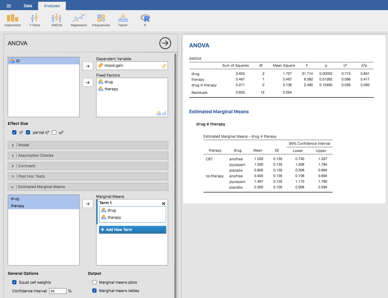
Fig. 151 jamovi screenshot showing the estimated marginal means for the saturated
model, i.e. including the interaction component, with the clinicaltrial
dataset
In the output we see that the estimated mean mood gain for the placebo group with no therapy was 0.300, with a 95% confidence interval from 0.006 to 0.594. Note that these are not the same confidence intervals that you would get if you calculated them separately for each group, because of the fact that the ANOVA model assumes homogeneity of variance and therefore uses a pooled estimate of the standard deviation.
When the model doesn’t contain the interaction term, then the estimated group
means will be different from the sample means. Instead of reporting the sample
mean, jamovi will calculate the value of the group means that would be expected
on the basis of the marginal means (i.e., assuming no interaction). Using the
notation we developed earlier, the estimate reported for µrc, the mean
for level r on the (row) Factor A and level c on the (column) Factor B
would be µ.. + αr + βc. If there are genuinely no
interactions between the two factors, this is actually a better estimate of the
population mean than the raw sample mean would be. Removing the interaction
term from the model, via the Model options in the jamovi ANOVA analysis,
provides the marginal means for the analysis shown in Fig. 152.
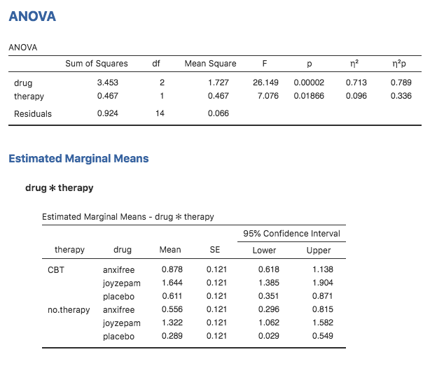
Fig. 152 jamovi screenshot showing the estimated marginal means for the unsaturated
model, i.e. without the interaction component, with the clinicaltrial
dataset
| [1] | This chapter seems to be setting a new record for the number of different things that the letter R can stand for. So far we have R referring to the software package, the number of rows in our table of means, the residuals in the model, and now the correlation coefficient in a regression. Sorry. We clearly don’t have enough letters in the alphabet. However, I’ve tried pretty hard to be clear on which thing R is referring to in each case. |
| [2] | Implausibly large, I would think. The artificiality of this data set is really starting to show! |