Section author: Danielle J. Navarro and David R. Foxcroft
Hypothesis tests for regression models
So far we’ve talked about what a regression model is, how the coefficients of a regression model are estimated, and how we quantify the performance of the model (the last of these, incidentally, is basically our measure of effect size). The next thing we need to talk about is hypothesis tests. There are two different (but related) kinds of hypothesis tests that we need to talk about: those in which we test whether the regression model as a whole is performing significantly better than a null model, and those in which we test whether a particular regression coefficient is significantly different from zero.
Testing the model as a whole
Okay, suppose you’ve estimated your regression model. The first hypothesis test you might try is the null hypothesis that there is no relationship between the predictors and the outcome, and the alternative hypothesis that the data are distributed in exactly the way that the regression model predicts.
Formally, our “null model” corresponds to the fairly trivial “regression” model in which we include 0 predictors and only include the intercept term b0:
If our regression model has K predictors, the “alternative model” is described using the usual formula for a multiple regression model:
How can we test these two hypotheses against each other? The trick is to understand that it’s possible to divide up the total variance SStot into the sum of the residual variance SSres and the regression model variance SSmod. I’ll skip over the technicalities, since we’ll get to that later when we look at ANOVA in chapter Comparing several means (one-way ANOVA). But just note that
And we can convert the sums of squares into mean squares by dividing by the degrees of freedom.
So, how many degrees of freedom do we have? As you might expect the df associated with the model is closely tied to the number of predictors that we’ve included. In fact, it turns out that dfmod = K. For the residuals the total degrees of freedom is dfres = N - K - 1.
Now that we’ve got our mean square values we can calculate an F-statistic like this
and the degrees of freedom associated with this are K and N - K - 1.
We’ll see much more of the F-statistic in chapter Comparing several means (one-way ANOVA), but for now just know that we can interpret large F-values as indicating that the null hypothesis is performing poorly in comparison to the alternative hypothesis. In a moment I’ll show you how to do the test in jamovi the easy way, but first let’s have a look at the tests for the individual regression coefficients.
Tests for individual coefficients
The F-test that we’ve just introduced is useful for checking that the model
as a whole is performing better than chance. If your regression model doesn’t
produce a significant result for the F-test then you probably don’t have a
very good regression model (or, quite possibly, you don’t have very good data).
However, while failing this test is a pretty strong indicator that the model
has problems, passing the test (i.e., rejecting the null) doesn’t imply that
the model is good! Why is that, you might be wondering? The answer to that can
be found by looking at the coefficients for the multiple regression model we
have already looked at Table 15 in section
Multiple linear regression above, where the coefficients we got were 125.966
(for the intercept), -8.950 (for dani.sleep) and 0.011 (for
baby.sleep). I can’t help but notice that the estimated regression
coefficient for the baby.sleep variable is tiny, relative to the value that
we get for dani.sleep. Given that these two variables are absolutely on the
same scale (they’re both measured in “hours slept”), I find this illuminating.
In fact, I’m beginning to suspect that it’s really only the amount of sleep
that I get that matters in order to predict my grumpiness.
We can re-use a hypothesis test that we discussed earlier, the t-test. The test that we’re interested in has a null hypothesis that the true regression coefficient is zero (b = 0), which is to be tested against the alternative hypothesis that it isn’t (b ≠ 0). That is:
How can we test this? Well, if the central limit theorem is kind to us we might be able to guess that the sampling distribution of \(\hat{b}\), the estimated regression coefficient, is a normal distribution with mean centred on b. What that would mean is that if the null hypothesis were true, then the sampling distribution of \(\hat{b}\) has mean zero and unknown standard deviation. Assuming that we can come up with a good estimate for the standard error of the regression coefficient, \(SE(\hat{b})\), then we’re in luck. That’s exactly the situation for which we introduced the one-sample t-test way back in chapter Comparing two means. So let’s define a t-statistic like this:
I’ll skip over the reasons why, but our degrees of freedom in this case are df = N - K - 1. Irritatingly, the estimate of the standard error of the regression coefficient, \(SE(\hat{b})\), is not as easy to calculate as the standard error of the mean that we used for the simpler t-tests in chapter Comparing two means. In fact, the formula is somewhat ugly, and not terribly helpful to look at.[1] For our purposes it’s sufficient to point out that the standard error of the estimated regression coefficient depends on both the predictor and outcome variables, and it is somewhat sensitive to violations of the homogeneity of variance assumption (discussed shortly).
In any case, this t-statistic can be interpreted in the same way as the t-statistics that we discussed in chapter Comparing two means. Assuming that you have a two-sided alternative (i.e., you don’t really care if b > 0 or b < 0), then it’s the extreme values of t (i.e., a lot less than zero or a lot greater than zero) that suggest that you should reject the null hypothesis.
Running the hypothesis tests in jamovi
To compute all of the statistics that we have talked about so far, all you need to do is make sure the relevant options are checked in jamovi and then run the regression. If we do that, as in Fig. 120, we get a whole bunch of useful output.
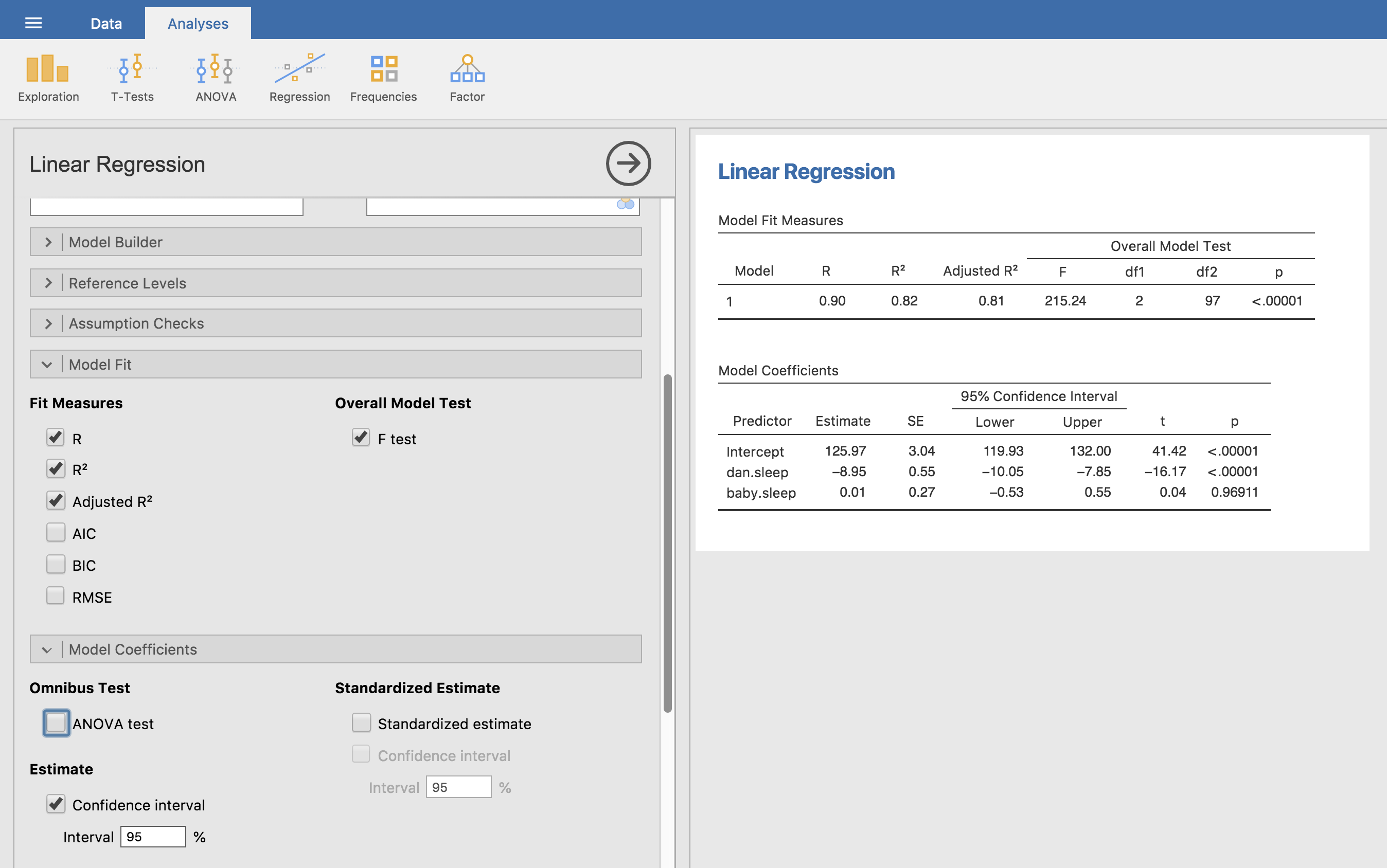
Fig. 120 jamovi screenshot showing a multiple linear regression analysis, with some useful options checked.
The Model Coefficients at the bottom of the jamovi analysis results shown
in Fig. 120 provides the coefficients of the regression model. Each
row in this table refers to one of the coefficients in the regression model.
The first row is the intercept term, and the later ones look at each of the
predictors. The columns give you all of the relevant information. The first
column is the actual estimate of b (e.g., 125.97 for the intercept, and
-8.95 for the dani.sleep predictor). The second column is the standard
error estimate \(\hat\sigma_b\). The third and fourth columns provide the
lower and upper values for the 95% confidence interval around the b
estimate (more on this later). The fifth column gives you the t-statistic,
and it’s worth noticing that in this table \(t= \hat{b}/ SE(\hat{b})\)
every time. Finally, the last column gives you the actual p-value for each
of these tests.[2]
The only thing that the coefficients table itself doesn’t list is the
degrees of freedom used in the t-test, which is always
N - K - 1 and is listed in the table at the top of the output,
labelled Model Fit Measures. We can see from this table that the model
performs significantly better than you’d expect by chance
(F(2,97) = 215.24, p < 0.001), which isn’t all that
surprising: the R² = 0.81 value indicate that the regression
model accounts for 81% of the variability in the outcome measure (and
82% for the adjusted R²). However, when we look back up at the
t-tests for each of the individual coefficients, we have pretty
strong evidence that the baby.sleep variable has no significant
effect. All the work in this model is being done by the dani.sleep
variable. Taken together, these results suggest that this regression
model is actually the wrong model for the data. You’d probably be better
off dropping the baby.sleep predictor entirely. In other words, the
simple regression model that we started with is the better model.
| [1] | For advanced readers only. The vector of residuals is \(\epsilon = y - X \hat{b}\). For K predictors plus the intercept, the estimated residual variance is \(\hat\sigma^2 = \epsilon^\prime\epsilon / (N - K - 1)\). The estimated covariance matrix of the coefficients is \(\hat\sigma^2(\mathbf{X}^\prime\mathbf{X})^{-1}\), the main diagonal of which is \(SE(\hat{b})\), our estimated standard errors. |
| [2] | Note that, although jamovi has done multiple tests here, it hasn’t done a Bonferroni correction or anything. These are standard one-sample t-tests with a two-sided alternative. If you want to make corrections for multiple tests, you need to do that yourself. |