Section author: Danielle J. Navarro and David R. Foxcroft
The McNemar test
Suppose you’ve been hired to work for the Australian Generic Political Party (AGPP), and part of your job is to find out how effective the AGPP political advertisements are. So you decide to put together a sample of N = 100 people and ask them to watch the AGPP ads. Before they see anything, you ask them if they intend to vote for the AGPP, and then after showing the ads you ask them again to see if anyone has changed their minds. Obviously, if you’re any good at your job, you’d also do a whole lot of other things too, but let’s consider just this one simple experiment. One way to describe your data is via the following contingency table:
| Before | After | Total | |
|---|---|---|---|
| Yes | 30 | 10 | 40 |
| No | 70 | 90 | 160 |
| Total | 100 | 100 | 200 |
At first pass, you might think that this situation lends itself to the Pearson χ² test of independence. However, a little bit of thought reveals that we’ve got a problem. We have 100 participants but 200 observations. This is because each person has provided us with an answer in both the before column and the after column. What this means is that the 200 observations aren’t independent of each other. If voter A says “yes” the first time and voter B says “no”, then you’d expect that voter A is more likely to say “yes” the second time than voter B! The consequence of this is that the usual χ² test won’t give trustworthy answers due to the violation of the independence assumption. Now, if this were a really uncommon situation, I wouldn’t be bothering to waste your time talking about it. But it’s not uncommon at all. This is a standard repeated measures design, and none of the tests we’ve considered so far can handle it. Eek.
The solution to the problem was published by McNemar (1947). The trick is to start by tabulating your data in a slightly different way:
| Before: Yes | Before: No | Total | |
|---|---|---|---|
| After: Yes | 5 | 5 | 10 |
| After: No | 25 | 65 | 90 |
| Total | 30 | 70 | 100 |
This is exactly the same data, but it’s been rewritten so that each of our 100 participants appears in only one cell. Because we’ve written our data this way the independence assumption is now satisfied, and this is a contingency table that we can use to construct a χ²-goodness-of-fit statistic. However, as we’ll see, we need to do it in a slightly non-standard way. To see what’s going on, it helps to label the entries in our table a little differently:
| Before: Yes | Before: No | Total | |
|---|---|---|---|
| After: Yes | a | b | a + b |
| After: No | c | d | c + d |
| Total | a + c | b + d | n |
Next, let’s think about what our null hypothesis is: it’s that the “before” test and the “after” test have the same proportion of people saying “Yes, I will vote for AGPP”. Because of the way that we have rewritten the data, it means that we’re now testing the hypothesis that the row totals and column totals come from the same distribution. Thus, the null hypothesis in McNemar’s test is that we have “marginal homogeneity”. That is, the row totals and column totals have the same distribution: Pa + Pb = Pa + Pc and similarly that Pc + Pd = Pb + Pd. Notice that this means that the null hypothesis actually simplifies to Pb = Pc. In other words, as far as the McNemar test is concerned, it’s only the off-diagonal entries in this table (i.e., b and c) that matter! After noticing this, the McNemar test of marginal homogeneity is no different to a usual χ² test. After applying the Yates correction, our test statistic becomes:
or, to revert to the notation that we used earlier in this chapter:
and this statistic has a χ² distribution (approximately) with df = 1. However, remember that just like the other χ² tests it’s only an approximation, so you need to have reasonably large expected cell counts for it to work.
Doing the McNemar test in jamovi
Now that you know what the McNemar test is all about, lets actually run one.
The agpp data set contains the raw data that I discussed previously. It
contains three variables, an id variable that labels each participant in
the dataset (we’ll see why that’s useful in a moment), a response_before
variable that records the person’s answer when they were asked the question the
first time, and a response_after variable that shows the answer that they
gave when asked the same question a second time. Notice that each participant
appears only once in this data set. Go to Analyses → Frequencies
→ Contingency Tables → Paired Samples in jamovi, and move
response_before into the Rows box, and response_after into the
Columns box. You will then get a contingency table in the results panel,
with the statistic for the McNemar test just below it (see
Fig. 80):
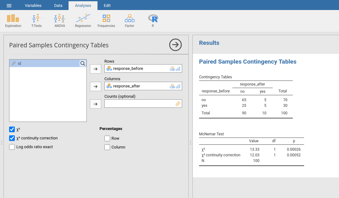
Fig. 80 McNemar test output in jamovi
And we’re done. We’ve just run a McNemar’s test to determine if people were just as likely to vote AGPP after the ads as they were before hand. The test was significant (χ²(1) = 12.03, p < 0.001), suggesting that they were not. And, in fact it looks like the ads had a negative effect: people were less likely to vote AGPP after seeing the ads. Which makes a lot of sense when you consider the quality of a typical political advertisement.
What’s the difference between McNemar and independence?
Let’s go all the way back to the beginning of the chapter and look at the
cards data set again. If you recall, the actual experimental design that I
described involved people making two choices. Because we have information
about the first choice and the second choice that everyone made, we can
construct the following contingency table that cross-tabulates the first choice
against the second choice.
          choice_2
choice_1   clubs diamonds hearts spades
  clubs       10        9     10      6
  diamonds    20        4     13     14
  hearts      20       18      3     23
  spades      18       13     15      4
Suppose I wanted to know whether the choice you make the second time is dependent on the choice you made the first time. This is where a test of independence is useful, and what we’re trying to do is see if there’s some relationship between the rows and columns of this table.
Alternatively, suppose I wanted to know if on average, the frequencies of suit choices were different the second time than the first time. In that situation, what I’m really trying to see is if the row totals are different from the column totals. That’s when you use the McNemar test.
The different statistics produced by these different analyses are shown in Fig. 81. Notice that the results are different! These aren’t the same test.
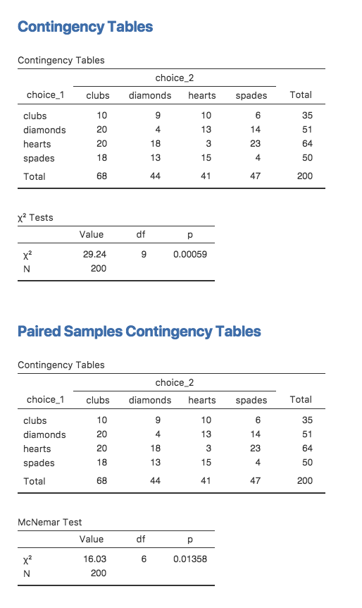
Fig. 81 Independent vs. Paired (McNemar) test output in jamovi