Section author: Danielle J. Navarro and David R. Foxcroft

Tabulating and cross-tabulating data

A very common task when analysing data is the construction of frequency tables, or cross-tabulation of one variable against another. These tasks can be achieved in jamovi and I’ll show you how in this section.

Creating tables for single variables

Let’s start with a simple example. As a parent of a small child I naturally spend a lot of time watching TV shows like In the Night Garden. In the nightgarden data set, I’ve transcribed a short section of the dialogue. The file contains two variables of interest, speaker and utterance. Open up this data set in jamovi and take a look at the data in the Data view. You will see that the data looks something like this:

speaker variable

upsy-daisy upsy-daisy upsy-daisy upsy-daisy tombliboo tombliboo makka-pakka makka-pakka makka-pakka makka-pakka

utterance variable

pip pip onk onk ee oo pip pip onk onk

Looking at this it becomes very clear what happened to my sanity! With these as my data, one task I might find myself needing to do is construct a frequency count of the number of words each character speaks during the show. The jamovi Descriptives screen has a check box called Frequency tables which does just this, see Fig. 32.

Fig. 32 Frequency table for the speaker variable

The output here tells us on the first line that what we’re looking at is a tabulation of the speaker variable. In the Levels column it lists all the different speakers that exist in the data, and in the Counts column it tells you how many times that speaker appears in the data. In other words, it’s a frequency table.

In jamovi, the Frequency tables check box will only produce a table for single variables. For a table of two variables, for example combining speaker and utterance so that we can see how many times each speaker said a particular utterance, we need a cross-tabulation or contingency table. In jamovi you can do this by selecting the Frequencies → Contingency Tables → Independent Samples analysis, and moving the speaker variable into the Rows box, and the utterance variable into the Columns box. You then should have a contingency table like the one shown in Fig. 33.

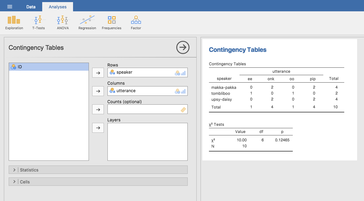
Fig. 33 Contingency table for the speaker and utterance variables

Don’t worry about the “χ² Tests” table that is produced. We are going to cover this later on in chapter Categorical data analysis. When interpreting the contingency table remember that these are counts, so the fact that the first row and second column of numbers corresponds to a value of 2 indicates that makka-pakka (row 1) says onk (column 2) twice in this data set.

Adding percentages to a contingency table

The contingency table shown in Fig. 33 shows a table of raw frequencies. That is, a count of the total number of cases for different combinations of levels of the specified variables. However, often you want your data to be organised in terms of percentages as well as counts. You can find the check boxes for different percentages under the Cells option in the Contingency Tables window. First, click on the Row check box and the Contingency Table in the output window will change to the one in Fig. 34.

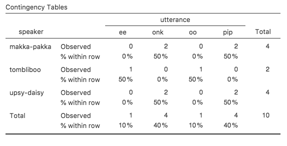
Fig. 34 Contingency table for the speaker and utterance variables, with row percentages

What we’re looking at here is the percentage of utterances made by each character. In other words, 50% of makka-pakka’s utterances are pip, and the other 50% are onk. Let’s contrast this with the table we get when we calculate column percentages (uncheck Row and check Column in the Cells options window), see Fig. 35. In this version, what we’re seeing is the percentage of characters associated with each utterance. For instance, whenever the utterance ee is made (in this data set), 100% of the time it’s a Tombliboo saying it.

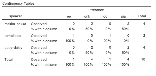
Fig. 35 Contingency table for the speaker and utterance variables, with column percentages