Section author: Danielle J. Navarro and David R. Foxcroft

Measures of variability

The statistics that we have discussed so far all relate to central tendency. That is, they all talk about which values are “in the middle” or “popular” in the data. However, central tendency is not the only type of summary statistic that we want to calculate. The second thing that we really want is a measure of the variability of the data. That is, how “spread out” are the data? How “far” away from the mean or median do the observed values tend to be? For now, let us assume that the data are interval or ratio scale, and we will continue to use the afl.margins variable. We will use this data to discuss several different measures of spread, each with different strengths and weaknesses.

Range

The range of a variable is very simple. It is the biggest value minus the smallest value. For the afl.margins variable the maximum value is 116 and the minimum value is 0. Although the range is the simplest way to quantify the notion of “variability”, it is one of the worst. Recall from our discussion of the mean that we want our summary measure to be robust. If the data set has one or two extremely bad values in it we would like our statistics to not be unduly influenced by these cases. For example, in a variable containing very extreme outliers, it is clear that the range is not robust. This variable has a range of 110 but if the outlier were removed we would have a range of only 8:

-100, 2, 3, 4, 5, 6, 7, 8, 9, 10

Interquartile range

The interquartile range (IQR) is like the range, but instead of the difference between the biggest and smallest value the difference between the 25th percentile and the 75th percentile is taken. If you do not already know what a percentile is, the 10th percentile of a data set is the smallest number x such that 10% of the data is less than x. In fact, we have already come across the idea. The median of a data set is its 50th percentile! In jamovi you can easily specify the 25th, 50th and 75th percentiles by clicking the checkbox Quartiles in the Exploration → Descriptives → Statistics screen.

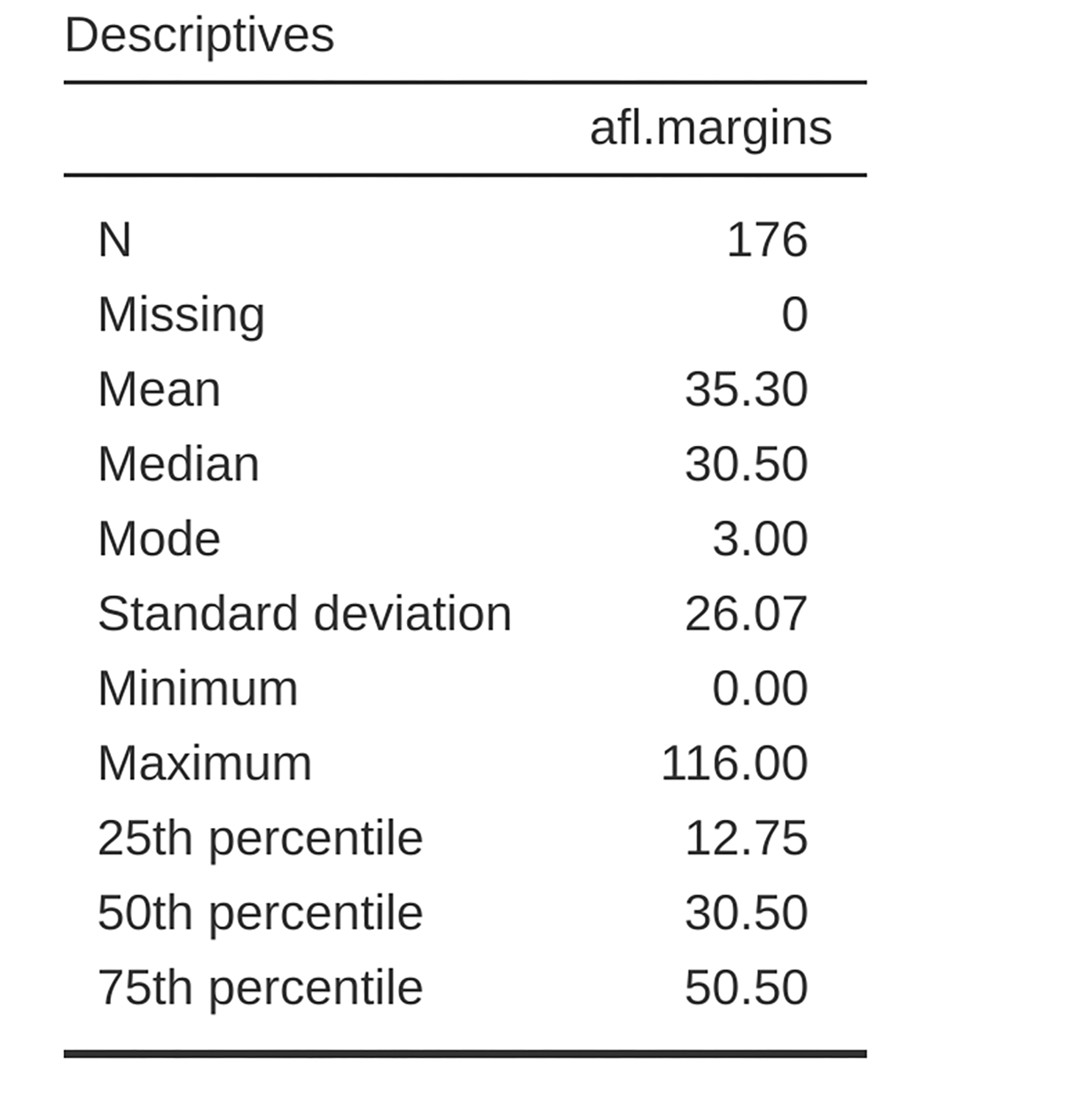
Fig. 13 Screenshot of jamovi showing the Quartiles for the afl.margins variable

Not surprisingly, in Fig. 13 the 50th percentile is the same as the median value. And, by noting that 50.50 - 12.75 = 37.75, we can see that the interquartile range for the afl.margins variable is 37.75. While it is obvious how to interpret the range it is a little less obvious how to interpret the IQR. The simplest way to think about it is like this: the interquartile range is the range spanned by the “middle half” of the data. That is, one quarter of the data falls below the 25th percentile and one quarter of the data is above the 75th percentile, leaving the “middle half” of the data lying in between the two. And the IQR is the range covered by that middle half.

Mean absolute deviation

The two measures we have looked at so far, the range and the interquartile range, both rely on the idea that we can measure the spread of the data by looking at the percentiles of the data. However, this is not the only way to think about the problem. A different approach is to select a meaningful reference point (usually the mean or the median) and then report the “typical” deviations from that reference point. What do we mean by “typical” deviation? Usually, this is the mean or median value of these deviations. In practice, this leads to two different measures: the “mean absolute deviation” (from the mean) and the “median absolute deviation” (from the median). From what I have read, the measure based on the median seems to be used in statistics and does seem to be the better of the two. But to be honest I do not think I have seen it used much in psychology. The measure based on the mean does occasionally show up in psychology though. In this section I will talk about the first one, and I will come back to talk about the second one later.

Since the previous paragraph might sound a little abstract, let us go through the mean absolute deviation from the mean a little more slowly. One useful thing about this measure is that the name actually tells you exactly how to calculate it. Let us think about our afl.margins variable, and once again we will start by pretending that there are only five games in total, with winning margins of 56, 31, 56, 8 and 32. Since our calculations rely on an examination of the deviation from some reference point (in this case the mean), the first thing we need to calculate is the mean, X̄. For these five observations, our mean is X̄ = 36.6. The next step is to convert each of our observations X_i into a deviation score. We do this by calculating the difference between the observation X_i and the mean X̄. That is, the deviation score is defined to be X_i - X̄. For the first observation in our sample, this is equal to 56 - 36.6 = 19.4. Okay, that is simple enough. The next step in the process is to convert these deviations to absolute deviations, and we do this by converting any negative values to positive ones. Mathematically, we would denote the absolute value of -3 as |-3|, and so we say that |-3| = 3. We use the absolute value here because we do not really care whether the value is higher than the mean or lower than the mean, we are just interested in how close it is to the mean. To help make this process as obvious as possible, the table below shows these calculations for all five observations:

Description:	which game	value	deviation from mean	absolute deviation
Notation:	i	Xi	Xi - X̄	| Xi - X̄ |
	1	56	19.4	19.4
	2	31	-5.6	5.6
	3	56	19.4	19.4
	4	8	-28.6	28.6
	5	32	-4.6	4.6

Now that we have calculated the absolute deviation score for every observation in the data set, all that we have to do to calculate the mean of these scores. Let us do that:

\[\frac{19.4 + 5.6 + 19.4 + 28.6 + 4.6}{5} = 15.52\]

And we are done. The mean absolute deviation for these five scores is 15.52.

However, whilst our calculations for this little example are at an end, we do have a couple of things left to talk about. First, we should really try to write down a proper mathematical formula. But in order do to this I need some mathematical notation to refer to the mean absolute deviation. Irritatingly, “mean absolute deviation” and “median absolute deviation” have the same acronym (MAD), which leads to a certain amount of ambiguity so I should better come up with something different for the mean absolute deviation. What I will do is use AAD instead, short for average absolute deviation. Now that we have some unambiguous notation, here is the formula that describes what we just calculated:

\[AAD(X) = \frac{1}{N} \sum_{i = 1}^N |X_i - \bar{X}|\]

Variance

Although the average absolute deviation measure has its uses, it is not the best measure of variability to use. From a purely mathematical perspective there are some solid reasons to prefer squared deviations rather than absolute deviations. If we do that we obtain a measure called the variance, which has a lot of really nice statistical properties that I am going to ignore,[1] and one massive psychological flaw that I am going to make a big deal out of in a moment. The variance of a data set X is sometimes written as Var(X), but it is more commonly denoted s² (the reason for this will become clearer shortly).

The formula that we use to calculate the variance of a set of observations is as follows:

\[\mbox{Var}(X) = \frac{1}{N} \sum_{i = 1} ^ N \left( X_i - \bar{X} \right) ^ 2\]

As you can see, it is basically the same formula that we used to calculate the average absolute deviation, except that instead of using “absolute deviations” we use “squared deviations”. It is for this reason that the variance is sometimes referred to as the “mean square deviation”.

Now that we have got the basic idea, let us have a look at a concrete example. Once again, let us use the first five AFL games as our data. If we follow the same approach that we took last time, we end up with the following table:

Description:	which game	value	deviation from mean	squared deviation
Notation:	i	Xi	Xi - X̄	(Xi - X̄)²
	1	56	19.4	376.36
	2	31	-5.6	31.36
	3	56	19.4	376.36
	4	8	-28.6	817.96
	5	32	-4.6	21.16

That last column contains all of our squared deviations, so all we have to do is average them. If we do that by hand, i.e., using a calculator, we end up with a variance of 324.64. Exciting, is not it? For the moment, let us ignore the burning question that you are all probably thinking (i.e., what the heck does a variance of 324.64 actually mean?) and instead talk a bit more about how to do the calculations in jamovi, because this will reveal something very weird. Start a new jamovi session by clicking on the main menu button (☰; top left-hand corner) and selecting New. Now type in the first five values from the aflsmall_margins data set in column A (56, 31, 56, 8, 32). Change the variable type to Continuous and under Descriptives click the Variance check box, and you get the same values for variance as the one we calculated by hand (324.64). No, wait, you get a completely different answer (405.80) – see Fig. 14.

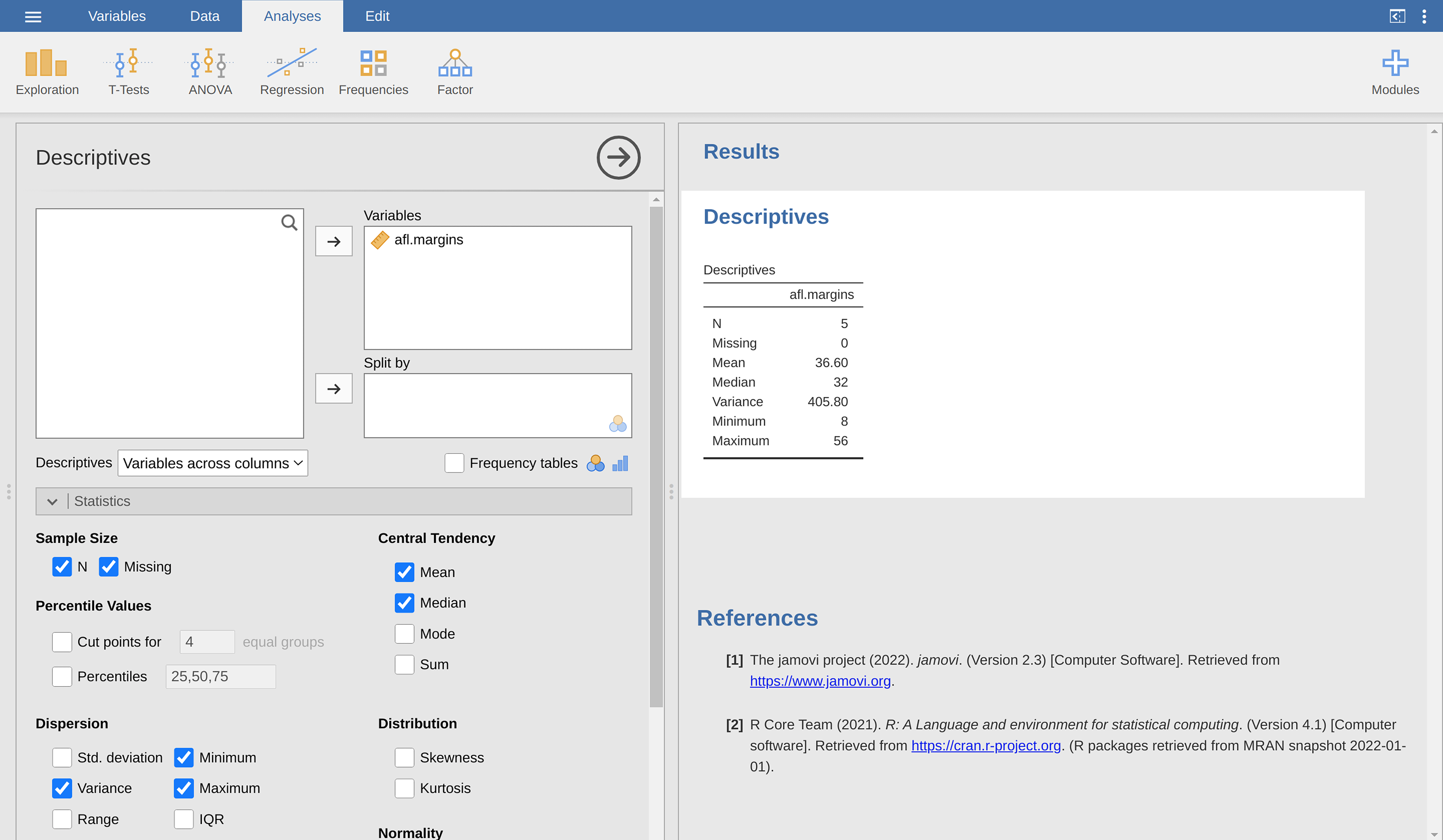
Fig. 14 Screenshot of jamovi showing the Variance for the first five values of the afl.margins variable

That is just weird – is jamovi broken? As it happens, the answer is no.[2] It is not a typo, and jamovi is not making a mistake. In fact, it is very simple to explain what jamovi is doing here, but slightly trickier to explain why jamovi is doing it. So let us start with the “what”. What jamovi is doing is evaluating a slightly different formula to the one I showed you above. Instead of averaging the squared deviations, which requires you to divide by the number of data points N, jamovi has chosen to divide by N - 1.

In other words, the formula that jamovi is using is this one:

\[\frac{1}{N - 1} \sum_{i = 1} ^ N \left( X_i - \bar{X} \right) ^ 2\]

So that is the what. The real question is why jamovi is dividing by N - 1 and not by N. After all, the variance is supposed to be the mean squared deviation, right? So should not we be dividing by N, the actual number of observations in the sample? Well, yes, we should. However, as we will discuss in chapter Estimating unknown quantities from a sample, there is a subtle distinction between “describing a sample” and “making guesses about the population from which the sample came”. Up to this point, it is been a distinction without a difference. Regardless of whether you are describing a sample or drawing inferences about the population, the mean is calculated exactly the same way. Not so for the variance, or the standard deviation, or for many other measures. What I outlined to you initially (i.e., take the actual average, and thus divide by N) assumes that you literally intend to calculate the variance of the sample. Most of the time, however, you are not terribly interested in the sample in and of itself. Rather, the sample exists to tell you something about the world. If so, you are actually starting to move away from calculating a “sample statistic” and towards the idea of estimating a “population parameter”. However, I am getting ahead of myself. For now, let us just take it on faith that jamovi knows what it is doing, and we will revisit the question later on when we talk about estimation.

Okay, one last thing. This section so far has read a bit like a mystery novel. I have shown you how to calculate the variance, described the weird “N - 1” thing that jamovi does and hinted at the reason why it is there, but I have not mentioned the single most important thing. How do you interpret the variance? Descriptive statistics are supposed to describe things, after all, and right now the variance is really just a gibberish number. Unfortunately, the reason why I have not given you the human-friendly interpretation of the variance is that there really is not one. This is the most serious problem with the variance. Although it has some elegant mathematical properties that suggest that it really is a fundamental quantity for expressing variation, it is completely useless if you want to communicate with an actual human. Variances are completely uninterpretable in terms of the original variable! All the numbers have been squared and they do not mean anything anymore. This is a huge issue. For instance, according to the table I presented earlier, the margin in game 1 was “376.36 points-squared higher than the average margin”. This is exactly as stupid as it sounds, and so when we calculate a variance of 324.64 we are in the same situation. I have watched a lot of footy games, and at no time has anyone ever referred to “points squared”. It is not a real unit of measurement, and since the variance is expressed in terms of this gibberish unit, it is totally meaningless to a human.

Standard deviation

Suppose that you like the idea of using the variance because of those nice mathematical properties that I have not talked about, but since you are a human and not a robot you would like to have a measure that is expressed in the same units as the data itself (i.e., points, not points-squared). What should you do? The solution to the problem is obvious! Take the square root of the variance, known as the standard deviation, also called the “root mean squared deviation”, or RMSD. This solves our problem fairly neatly. Whilst no-one has a clue what “a variance of 324.68 points-squared” really means, it is much easier to understand “a standard deviation of 18.01 points” since it is expressed in the original units. It is traditional to refer to the standard deviation of a sample of data as s, though “SD”, “sd” and “std dev.” are also used at times.

Because the standard deviation is equal to the square root of the variance, you probably will not be surprised to see that the formula is:

\[s = \sqrt{ \frac{1}{N} \sum_{i = 1} ^ N \left( X_i - \bar{X} \right) ^ 2 }\]

and in jamovi there is a check box for Std. deviation right above the check box for Variance. Selecting this gives a value of 26.07 for the standard deviation.

However, as you might have guessed from our discussion of the variance, what jamovi actually calculates is slightly different to the formula given above. Just like we saw with the variance, what jamovi calculates is a version that divides by N - 1 rather than N.

For reasons that will make sense when we return to this topic in chapter Estimating unknown quantities from a sample I will refer to this new quantity as \(\hat\sigma\) (read as: “sigma hat”), and the formula for this is:

\[\hat\sigma = \sqrt{ \frac{1}{N - 1} \sum_{i = 1} ^ N \left( X_i - \bar{X} \right) ^ 2 }\]

Interpreting standard deviations is slightly more complex. Because the standard deviation is derived from the variance, and the variance is a quantity that has little to no meaning that makes sense to us humans, the standard deviation does not have a simple interpretation. As a consequence, most of us just rely on a simple rule of thumb. In general, you should expect 68% of the data to fall within one standard deviation of the mean, 95% of the data to fall within two standard deviation of the mean, and 99.7% of the data to fall within three standard deviations of the mean. This rule tends to work pretty well most of the time, but it is not exact. It is actually calculated based on an assumption that the histogram is symmetric and “bell shaped”.[3] As you can tell from looking at the histogram for the afl.margins variable in Fig. 21, this is not exactly true of our data! Even so, the rule is approximately correct. As it turns out, 65.3% of the data in the afl.margins variable fall within one standard deviation of the mean. This is shown visually in Fig. 15.

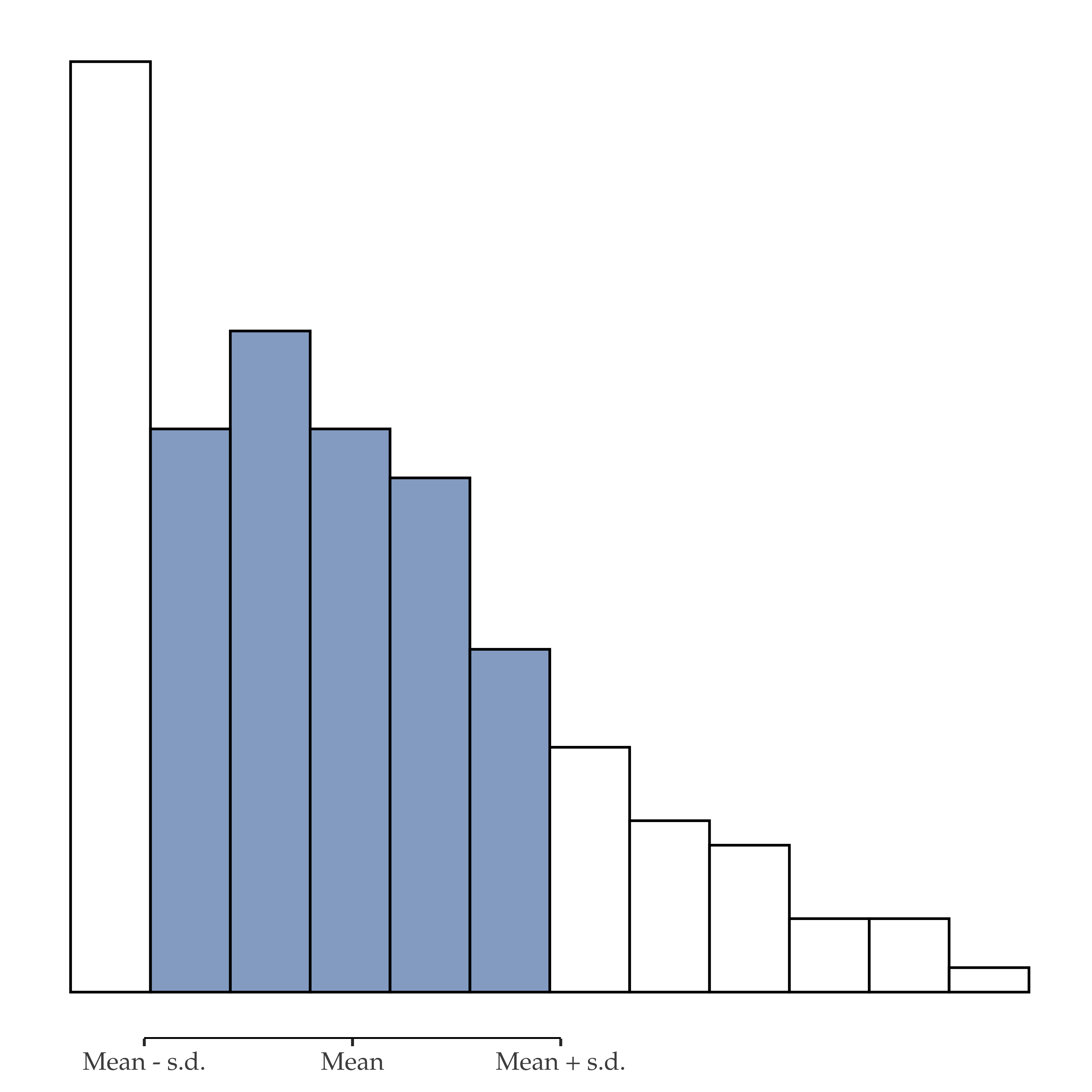
Fig. 15 Illustration of the standard deviation of the afl.margins variable. The shaded bars in the histogram show how much of the data fall within one standard deviation of the mean. In this case, 65.3% of the data set lies within this range, which is pretty consistent with the “approximately 68% rule” discussed in the main text.

Which measure to use?

We have discussed quite a few measures of spread: range, IQR, mean absolute deviation, variance and standard deviation; and hinted at their strengths and weaknesses. Here is a quick summary:

• Range. Gives you the full spread of the data. It is very vulnerable to outliers and as a consequence it is not often used unless you have good reasons to care about the extremes in the data.

• Interquartile range. Tells you where the “middle half” of the data sits. It is pretty robust and complements the median nicely. This is used a lot.

• Mean absolute deviation. Tells you how far “on average” the observations are from the mean. It is very interpretable but has a few minor issues (not discussed here) that make it less attractive to statisticians than the standard deviation. Used sometimes, but not often.

• Variance. Tells you the average squared deviation from the mean. It is mathematically elegant and is probably the “right” way to describe variation around the mean, but it is completely uninterpretable because it does not use the same units as the data. Almost never used except as a mathematical tool, but it is buried “under the hood” of a very large number of statistical tools.

• Standard deviation. This is the square root of the variance. It is fairly elegant mathematically and it is expressed in the same units as the data so it can be interpreted pretty well. In situations where the mean is the measure of central tendency, this is the default. This is by far the most popular measure of variation.

In short, the IQR and the standard deviation are easily the two most common measures used to report the variability of the data. But there are situations in which the others are used. I have described all of them in this book because there is a fair chance you will run into most of these somewhere.

---

[1]

Well, I will very briefly mention the one that I think is coolest, for a very particular definition of “cool”, that is. Variances are additive. Here is what that means. Suppose I have two variables X and Y, whose variances are Var(X) and Var(Y) respectively. Now imagine I want to define a new variable Z that is the sum of the two, Z = X + Y. As it turns out, the variance of Z is equal to Var(X) + Var(Y). This is a very useful property, but it is not true of the other measures that I talk about in this section.

[2]

With the possible exception of the third question.

[3]

Strictly, the assumption is that the data are normally distributed, which is an important concept that we will discuss more in chapter Introduction to probability and will turn u over and over again later in the book.