Afsnitsforfatter: Danielle J. Navarro and David R. Foxcroft

Factorial ANOVA 1: balanced designs, no interactions

When we discussed analysis of variance in chapter Comparing several means (one-way ANOVA), we assumed a fairly simple experimental design. Each person is in one of several groups and we want to know whether these groups have different mean scores on some outcome variable. In this section, I will discuss a broader class of experimental designs known as factorial designs, in which we have more than one grouping variable . I gave one example of how this kind of design might arise above. Another example appears in chapter Comparing several means (one-way ANOVA) in which we were looking at the effect of different drugs on the mood.gain experienced by each person . In that chapter we did find a significant effect of drug, but at the end of the chapter we also ran an analysis to see if there was an effect of therapy. We did not find one, but there is something a bit worrying about trying to run two separate analyses trying to predict the same outcome. Maybe there actually is an effect of therapy on mood gain, but we could not find it because it was being “hidden” by the effect of drug? In other words, we are going to want to run a single analysis that includes both drug and therapy as predictors. For this analysis each person is cross-classified by the drug they were given (a factor with 3 levels) and what therapy they received (a factor with 2 levels). We refer to this as a 3 × 2 factorial design.

If we cross-tabulate drug by therapy, using the Frequencies → Contingency Tables analysis in jamovi (see Tabulating and cross-tabulating data), we get the table shown in figur 166.

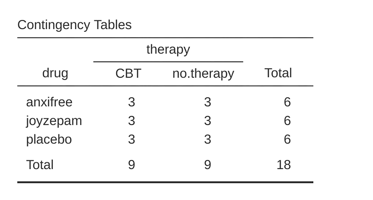
figur 166 jamovi contingency table for drug by therapy

As you can see, not only do we have participants corresponding to all possible combinations of the two factors, indicating that our design is completely crossed, it turns out that there are an equal number of people in each group. In other words, we have a balanced design. In this section I will talk about how to analyse data from balanced designs, since this is the simplest case. The story for unbalanced designs is quite tedious, so we will put it to one side for the moment.

What hypotheses are we testing?

Like one-way ANOVA, factorial ANOVA is a tool for testing certain types of hypotheses about population means. So a sensible place to start would be to be explicit about what our hypotheses actually are. However, before we can even get to that point, it is really useful to have some clean and simple notation to describe the population means. Because of the fact that observations are cross-classified in terms of two different factors, there are quite a lot of different means that one might be interested in. To see this, let us start by thinking about all the different sample means that we can calculate for this kind of design. Firstly, there is the obvious idea that we might be interested in this list of group means:

drug     therapy     mood.gain
placebo  no.therapy  0.300000
anxifree no.therapy  0.400000
joyzepam no.therapy  1.466667
placebo     CBT      0.600000
anxifree    CBT      1.033333
joyzepam    CBT      1.500000

Now, this output shows a list of the group means for all possible combinations of the two factors (e.g., people who received the placebo and no therapy, people who received the placebo while getting CBT, etc.). It is helpful to organise all these numbers, plus the marginal and grand means, into a single table:

	no therapy	CBT	total
placebo	0.30	0.60	0.45
anxifree	0.40	1.03	0.72
joyzepam	1.47	1.50	1.48
total	0.72	1.04	0.88

Now, each of these different means is of course a sample statistic. It is a quantity that pertains to the specific observations that we have made during our study. What we want to make inferences about are the corresponding population parameters. That is, the true means as they exist within some broader population. Those population means can also be organised into a similar table, but we will need a little mathematical notation to do so. As usual, I will use the symbol µ to denote a population mean. However, because there are lots of different means, I will need to use subscripts to distinguish between them.

Here is how the notation works. Our table is defined in terms of two factors. Each row corresponds to a different level of factor A (in this case drug), and each column corresponds to a different level of factor B (in this case therapy). If we let R denote the number of rows in the table, and C denote the number of columns, we can refer to this as an R × C factorial ANOVA. In this case R = 3 and C = 2. We will use lowercase letters to refer to specific rows and columns, so µ_rc refers to the population mean associated with the rth level of factor A (i.e., row number r) and the c-th level of factor B (i.e., column number c).[1] So the population means are now written like this:

	no therapy	CBT	total
placebo	µ11	µ11
anxifree	µ21	µ11
joyzepam	µ31	µ11
total

What about the remaining entries? For instance, how should we describe the average mood gain across the entire (hypothetical) population of people who might be given Joyzepam in an experiment like this, regardless of whether they were in CBT? We use the “dot” notation to express this. In the case of Joyzepam, notice that we are talking about the mean associated with the third row in the table. That is, we are averaging across two cell means (i.e., µ₃₁ and µ₃₂). The result of this averaging is referred to as a marginal mean, and would be denoted µ_3. in this case. The marginal mean for CBT corresponds to the population mean associated with the second column in the table, so we use the notation µ_.2 to describe it. The grand mean is denoted µ_.. because it is the mean obtained by averaging (marginalising[2]) over both. So our full table of population means can be written down like this:

	no therapy	CBT	total
placebo	µ11	µ12	µ1.
anxifree	µ21	µ22	µ2.
joyzepam	µ31	µ32	µ3.
total	µ.1	µ.2	µ..

Now that we have this notation, it is straightforward to formulate and express some hypotheses. Let us suppose that the goal is to find out two things. First, does the choice of drug have any effect on mood? And second, does CBT have any effect on mood? These are not the only hypotheses that we could formulate of course, and we will see a really important example of a different kind of hypothesis in section Factorial ANOVA 2: balanced designs, interactions allowed, but these are the two simplest hypotheses to test, and so we will start there. Consider the first test. If the drug has no effect then we would expect all of the row means to be identical, right? So that is our null hypothesis. On the other hand, if the drug does matter then we should expect these row means to be different. Formally, we write down our null and alternative hypotheses in terms of the equality of marginal means:

Null hypothesis, H0:	row means are the same, i.e., µ1. = µ2. = µ3.
Alternative hypothesis, H1:	at least one row mean is different

It is worth noting that these are exactly the same statistical hypotheses that we formed when we ran a one-way ANOVA on these data back in the previous chapter. Back then, I used the notation µ_P to refer to the mean mood gain for the placebo group, with µ_A and µ_J corresponding to the group means for the two drugs, and the null hypothesis was µ_P = µ_A = µ_J. So we are actually talking about the same hypothesis, it is just that the more complicated ANOVA requires more careful notation due to the presence of multiple grouping variables, so we are now referring to this hypothesis as µ_1. = µ_2. = µ_3.. However, as we will see shortly, although the hypothesis is identical the test of that hypothesis is subtly different due to the fact that we are now acknowledging the existence of the second grouping variable.

Speaking of the other grouping variable, you will not be surprised to discover that our second hypothesis test is formulated the same way. However, since we are talking about the psychological therapy rather than drugs our null hypothesis now corresponds to the equality of the column means:

Null hypothesis, H0:	column means are the same, i.e., µ.1 = µ.2
Alternative hypothesis, H1:	column means are different, i.e., µ.1 ≠ µ.2

Running the analysis in jamovi

The null and alternative hypotheses that I described in the last section should seem awfully familiar. They are basically the same as the hypotheses that we were testing in our simpler one-way ANOVAs. So you are probably expecting that the hypothesis tests that are used in factorial ANOVA will be essentially the same as the F-test from the previous chapter. You are expecting to see references to sums of squares (SS), mean squares (MS), degrees of freedom (df), and finally an F-statistic that we can convert into a p-value, right? Well, you are absolutely and completely right. So much so that I am going to depart from my usual approach. Throughout this book, I have generally taken the approach of describing the logic (and to an extent the mathematics) that underpins a particular analysis first and only then introducing the analysis in jamovi. This time I am going to do it the other way around and show you how to do it in jamovi first. The reason for doing this is that I want to highlight the similarities between the simpler one-Way ANOVA that we discussed in the previous chapter, and the more complicated approach that we are going to use in this chapter.

If the data you are trying to analyse correspond to a balanced factorial design then running your analysis of variance is easy. To see how easy it is, let us start by reproducing the original analysis from chapter Comparing several means (one-way ANOVA). In case you have forgotten, for that analysis we were using only a single factor (i.e., drug) to predict our outcome variable (i.e., mood.gain), and we got the results shown in figur 167.

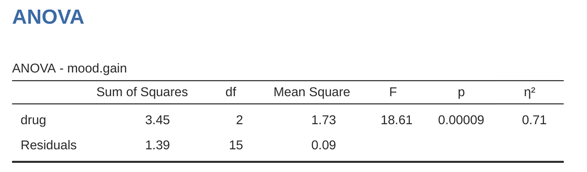
figur 167 jamovi One-way ANOVA of mood.gain by drug

Now, suppose I am also curious to find out if therapy has a relationship to mood.gain. In light of what we have seen from our discussion of multiple regression in chapter Correlation and linear regression, you probably will not be surprised that all we have to do is add therapy as a second Fixed Factor in the analysis, see figur 168.

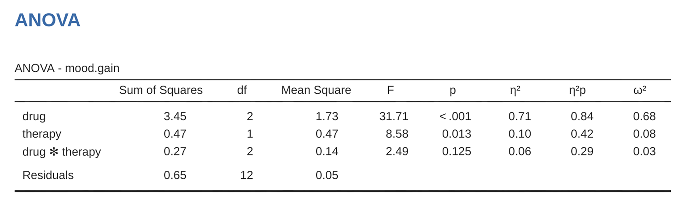
figur 168 jamovi factorial ANOVA for mood.gain with the two factors drug and therapy

This output is pretty simple to read too. The first row of the table reports a between-group sum of squares (SS) value associated with the drug factor, along with a corresponding between-group df-value. It also calculates a mean square value (MS), an F-statistic and a p-value. There is also a row corresponding to the therapy factor and a row corresponding to the residuals (i.e., the within groups variation).

Not only are all of the individual quantities pretty familiar, the relationships between these different quantities has remained unchanged, just like we saw with the original one-way ANOVA. Note that the mean square value is calculated by dividing SS by the corresponding df. That is, it is still true that:

MS = SS / df

regardless of whether we are talking about drug, therapy or the residuals. To see this, let us not worry about how the sums of squares values are calculated. Instead, let us take it on faith that jamovi has calculated the SS values correctly, and try to verify that all the rest of the numbers make sense. First, note that for the drug factor, we divide 3.45 by 2 and end up with a mean square value of 1.73. For the therapy factor, there is only 1 degree of freedom, so our calculations are even simpler: dividing 0.47 (the SS value) by 1 gives us an answer of 0.47 (the MS value).

Turning to the F-statistics and the p-values, notice that we have two of each; one corresponding to the drug factor and the other corresponding to the therapy factor. Regardless of which one we are talking about, the F-statistic is calculated by dividing the mean square value associated with the factor by the mean square value associated with the residuals. If we use “A” as shorthand notation to refer to the first factor (factor A; in this case drug) and “R” as shorthand notation to refer to the residuals, then the F-statistic associated with factor A is denoted F_A, and is calculated as follows:

F_A = MS_A / MS_R

and an equivalent formula exists for factor B (i.e., therapy). Note that this use of “R” to refer to residuals is a bit awkward, since we also used the letter R to refer to the number of rows in the table, but I am only going to use “R” to mean residuals in the context of SS_R and MS_R, so hopefully this should not be confusing. Anyway, to apply this formula to the drug factor we take the mean square of 1.73 and divide it by the residual mean square value of 0.07, which gives us an F-statistic of 26.15. The corresponding calculation for the therapy variable would be to divide 0.47 by 0.07 which gives 7.08 as the F-statistic. Not surprisingly, of course, these are the same values that jamovi has reported in the ANOVA table above.

Also in the ANOVA table is the calculation of the p-values. Once again, there is nothing new here. For each of our two factors what we are trying to do is test the null hypothesis that there is no relationship between the factor and the outcome variable (I will be a bit more precise about this later on). To that end, we have (apparently) followed a similar strategy to what we did in the One-Way ANOVA and have calculated an F-statistic for each of these hypotheses. To convert these to p-values, all we need to do is note that the sampling distribution for the F-statistic under the null hypothesis (that the factor in question is irrelevant) is an F- distribution. Also note that the two degrees of freedom values are those corresponding to the factor and those corresponding to the residuals. For the drug factor we are talking about an F- distribution with 2 and 14 degrees of freedom (I will discuss degrees of freedom in more detail later). In contrast, for the therapy factor the sampling distribution is F with 1 and 14 degrees of freedom.

At this point, I hope you can see that the ANOVA table for this more complicated factorial analysis should be read in much the same way as the ANOVA table for the simpler one-way analysis. In short, it is telling us that the factorial ANOVA for our 3 × 2 design found a significant effect of drug: F(2,14) = 26.15, p < 0.001, as well as a significant effect of therapy: F(1,14) = 7.08, p = 0.02. Or, to use the more technically correct terminology, we would say that there are two main effects of drug and therapy. At the moment, it probably seems a bit redundant to refer to these as “main” effects, but it actually does make sense. Later on, we are going to want to talk about the possibility of “interactions” between the two factors, and so we generally make a distinction between main effects and interaction effects.

How are the sum of squares calculated?

In the previous section I had two goals. Firstly, to show you that the jamovi method needed to do factorial ANOVA is pretty much the same as what we used for a One-Way ANOVA. The only difference is the addition of a second factor. Secondly, I wanted to show you what the ANOVA table looks like in this case, so that you can see from the outset that the basic logic and structure behind factorial ANOVA is the same as that which underpins One-Way ANOVA. Try to hold onto that feeling. It is genuinely true, insofar as factorial ANOVA is built-in more or less the same way as the simpler one-way ANOVA model. It is just that this feeling of familiarity starts to evaporate once you start digging into the details. Traditionally, this comforting sensation is replaced by an urge to hurl abuse at the authors of statistics textbooks.

Okay, let us start by looking at some of those details. The explanation that I gave in the last section illustrates the fact that the hypothesis tests for the main effects (of drug and therapy in this case) are F-tests, but what it does not do is show you how the sum of squares (SS) values are calculated. Nor does it tell you explicitly how to calculate degrees of freedom (df-values) though that is a simple thing by comparison. Let us assume for now that we have only two predictor variables, factor A and factor B. If we use Y to refer to the outcome variable, then we would use Y_rci to refer to the outcome associated with the i-th member of group rc (i.e., level / row r for factor A and level / column c for factor B). Thus, if we use Ȳ to refer to a sample mean, we can use the same notation as before to refer to group means, marginal means and grand means. That is, Ȳ_rc is the sample mean associated with the rth level of factor A and the cth level of factor B, Ȳ_r. would be the marginal mean for the rth level of factor A, Ȳ_.c would be the marginal mean for the cth level of factor B, and Ȳ_.. is the grand mean. In other words, our sample means can be organised into the same table as the population means. For our clinicaltrial data, that table looks like this:

	no therapy	CBT	total
placebo	Ȳ11	Ȳ12	Ȳ1.
anxifree	Ȳ21	Ȳ22	Ȳ2.
joyzepam	Ȳ31	Ȳ32	Ȳ3.
total	Ȳ.1	Ȳ.2	Ȳ..

And if we look at the sample means that I showed earlier, we have Ȳ₁₁ = 0.30, Ȳ₁₂ = 0.60 etc. In our clinicaltrial data, the drug factor has 3 levels and the therapy factor has 2 levels, and so what we are trying to run is a 3 × 2 factorial ANOVA. However, we will be a little more general and say that factor A (the row factor) has r levels and factor B (the column factor) has c levels, and so what we are runnning here is an r × c factorial ANOVA.

Now that we have got our notation straight, we can compute the sum of squares values for each of the two factors in a relatively familiar way. For factor A, our between group sum of squares is calculated by assessing the extent to which the (row) marginal means Ȳ_1., Ȳ_2. etc, are different from the grand mean Ȳ_... We do this in the same way that we did for one-way ANOVA: calculate the sum of squared difference between the Ȳ_i. values and the Ȳ_.. values. Specifically, if there are N people in each group, then we calculate this:

\[\mbox{SS}_{A} = (N \times C) \sum_{r = 1} ^ R \left( \bar{Y}_{r.} - \bar{Y}_{..} \right) ^ 2\]

As with one-way ANOVA, the most interesting[3] part of this formula is the (Ȳ_r. – Ȳ_..)² bit, which corresponds to the squared deviation associated with level r. All that this formula does is calculate this squared deviation for all R levels of the factor, add them up, and then multiply the result by N × C. The reason for this last part is that there are multiple cells in our design that have level r on factor A. In fact, there are C of them, one corresponding to each possible level of factor B! For instance, in our example there are two different cells in the design corresponding to the anxifree drug: one for people with no.therapy and one for the CBT group. Not only that, within each of these cells there are N observations. So, if we want to convert our SS value into a quantity that calculates the between-groups sum of squares on a “per observation” basis, we have to multiply by N × C. The formula for factor B is of course the same thing, just with some subscripts shuffled around:

\[\mbox{SS}_{B} = (N \times R) \sum_{c = 1} ^ C \left( \bar{Y}_{.c} - \bar{Y}_{..} \right) ^ 2\]

Now that we have these formulas we can check them against the jamovi output from the earlier section.

First, let us calculate the sum of squares associated with the main effect of drug. There are a total of N = 3 people in each group and C = 2 different types of therapy. Or, to put it another way, there are 3 · 2 = 6 people who received any particular drug. When we do these calculations in a spreadsheet programme, we get a value of 3.45 for the sum of squares associated with the main effect of drug. Not surprisingly, this is the same number that you get when you look up the SS value for the drug factor in the ANOVA table that I presented earlier, in figur 168.

We can repeat the same kind of calculation for the effect of therapy. Again, there are N = 3 people in each group, but since there are R = 3 different values in drug, this time around we note that there are 3 · 3 = 9 people who received CBT and an additional 9 people who received no.therapy. So our calculation in this case gives us a value of 0.47 for the sum of squares associated with the main effect of therapy. Once again, we are not surprised to see that our calculations are identical to the ANOVA output in figur 168.

So that is how you calculate the SS values for the two main effects. These SS values are analogous to the between-group sum of squares values that we calculated when doing the one-way ANOVA in the previous chapter. However, it is not a good idea to think of them as between-groups SS values anymore, just because we have two different grouping variables and it is easy to get confused. In order to construct an F-test, however, we also need to calculate the within-groups sum of squares. In keeping with the terminology that we used in chapter Correlation and linear regression and the terminology that jamovi uses when printing out the ANOVA table, I will start referring to the within-groups SS value as the residual sum of squares SS_R.

The easiest way to think about the residual SS values in this context, I think, is to think of it as the leftover variation in the outcome variable after you take into account the differences in the marginal means (i.e., after you remove SS_A and SS_B). What I mean by that is we can start by calculating the total sum of squares, which I will label SS_T. The formula for this is pretty much the same as it was for one-way ANOVA. We take the difference between each observation Y_rci and the grand mean Ȳ_.., square the differences, and add them all up

\[\mbox{SS}_T = \sum_{r = 1} ^ R \sum_{c = 1} ^ C \sum_{i = 1} ^ N \left( Y_{rci} - \bar{Y}_{..}\right) ^ 2\]

The “triple summation” here looks more complicated than it is. In the first two summations, we are summing across all levels of factor A (i.e., over all possible rows r in our table) and across all levels of factor B (i.e., all possible columns c). Each rc-combination corresponds to a single group and each group contains N people, so we have to sum across all those people (i.e., all i values) too. In other words, all we are doing here is summing across all observations in the data set (i.e., all possible rci-combinations).

At this point, we know the total variability of the outcome variable SS_T, and we know how much of that variability can be attributed to factor A (SS_A) and how much of it can be attributed to factor B (SS_B). The residual sum of squares is thus defined to be the variability in Y that can not be attributed to either of our two factors. In other words

SS_R = SS_T - (SS_A + SS_B)

Of course, there is a formula that you can use to calculate the residual SS (SS_R) directly, but I think that it makes more conceptual sense to think of it like this. The whole point of calling it a residual is that it is the leftover variation, and the formula above makes that clear. I should also note that, in keeping with the terminology used in the regression chapter, it is commonplace to refer to SS_A + SS_B as the variance attributable to the “ANOVA model”, denoted SS_M, and so we often say that the total sum of squares is equal to the model sum of squares plus the residual sum of squares. Later on in this chapter we will see that this is not just a surface similarity: ANOVA and regression are actually the same thing under the hood.

In any case, it is probably worth taking a moment to check that we can calculate SS_R using this formula and verify that we do obtain the same answer that jamovi produces in its ANOVA table. The calculations are pretty straightforward when done using computed variables in jamovi. We download and open the clinicaltrial data set and define three computed variables: (1) sq_res_T with (mood.gain - VMEAN(mood.gain)) ^ 2 as formula, (2) sq_res_A with (VMEAN(mood.gain) - VMEAN(mood.gain, group_by = drug)) ^ 2 as formula, and (3) sq_res_B with (VMEAN(mood.gain) - VMEAN(mood.gain, group_by = therapy)) ^ 2 as formula. Once we created those three variables, we calculate the sum of squares using Descriptives → Descriptive Statistics, then moving sq_res_T, sq_res_A and sq_res_B to the Variables box, and finally selecting Sum from the Statistics drop-down menu. SS_T (sq_res_T) has a value of 4.845, SS_A (sq_res_A) a value of 3.453, and SS_B (sq_res_B) a value of 0.467. Using these three values, we can calculate SS_R using the formula above.

SS_R = 4.845 - (3.453 + 0.467)

SS_R = 0.924

Alternatively, we can create another computed variable with the name SS_R and the formula VSUM(sq_res_T) - (VSUM(sq_res_A) + VSUM(sq_res_B)).

What are our degrees of freedom?

The degrees of freedom are calculated in much the same way as for one-way ANOVA. For any given factor, the degrees of freedom is equal to the number of levels minus 1 (i.e., R - 1 for the row variable factor A, and C - 1 for the column variable factor B). So, for the drug factor we obtain df = 2, and for the therapy factor we obtain df = 1. Later on, when we discuss the interpretation of ANOVA as a regression model (see section ANOVA as a linear model), I will give a clearer statement of how we arrive at this number. But for the moment we can use the simple definition of degrees of freedom, namely that the degrees of freedom equals the number of quantities that are observed, minus the number of constraints. So, for the drug factor, we observe three separate group means, but these are constrained by one grand mean, and therefore the degrees of freedom is 2. For the residuals, the logic is similar, but not quite the same. The total number of observations in our experiment is 18. The constraints correspond to one grand mean, the two additional group means that the drug factor introduces, and the one additional group mean that the the therapy factor introduces, and so our degrees of freedom is 14. As a formula, this is N - 1 - (R - 1) - (C - 1), which simplifies to N - R - C + 1.

Using the degrees of freedom and the square sums we calculated above, we can calculate the following F-values for the factors A and B.

F_A = (SS_A / df_A) / (SS_R / df_R)

F_A = (3.453 / 2) / (0.924 / 14)

F_A = 1.727 / 0.066

F_A = 26.149

F_B = (SS_B / df_B) / (SS_R / df_R)

F_B = (0.467 / 1) / (0.924 / 14)

F_B = 0.467 / 0.066

F_B = 7.076

Again, we can also create two new computed variables, the first with the name F_A and the formula (VSUM(sq_res_A) / 2) / (SS_R / 14), and the second with the name F_B and the formula (VSUM(sq_res_B) / 1) / (SS_R / 14).

Those, who don’t want to have a go themselves or can’t reproduce the calculations described in the previous paragraphs can download and open the clinicaltrial_factorialanova data set and look at the calculations there.

Factorial ANOVA versus one-way ANOVAs

Now that we have seen how a factorial ANOVA works, it is worth taking a moment to compare it to the results of the one-way analyses, because this will give us a really good sense of why it is a good idea to run the factorial ANOVA. In chapter Comparing several means (one-way ANOVA), I ran a one-way ANOVA that looked to see if there are any differences between the three levels of drug, and a second one-way ANOVA to see if there were any differences between the two levels of therapy. As we saw in section What hypotheses are we testing?, the null and alternative hypotheses tested by the one-way ANOVAs are in fact identical to the hypotheses tested by the factorial ANOVA. Looking even more carefully at the ANOVA tables, we can see that the sum of squares associated with the factors are identical in the two different analyses (3.453 for drug and 0.467 for therapy), as are the degrees of freedom (2 for drug, 1 for therapy). But they do not give the same answers! Most notably, when we ran the one-way ANOVA for therapy in section On the relationship between ANOVA and the Student t-test we did not find a significant effect (the p-value was 0.210). However, when we look at the main effect of therapy within the context of the two-way ANOVA, we do get a significant effect (p = 0.019). The two analyses are clearly not the same.

Why does that happen? The answer lies in understanding how the residuals are calculated. Recall that the whole idea behind an F-test is to compare the variability that can be attributed to a particular factor with the variability that cannot be accounted for (the residuals). If you run a one-way ANOVA for therapy, and therefore ignore the effect of drug, the ANOVA will end up dumping all of the drug-induced variability into the residuals! This has the effect of making the data look more noisy than they really are, and the effect of therapy which is correctly found to be significant in the two-way ANOVA now becomes non-significant. If we ignore something that actually matters (e.g., drug) when trying to assess the contribution of something else (e.g., therapy) then our analysis will be distorted. Of course, it is perfectly okay to ignore variables that are genuinely irrelevant to the phenomenon of interest. If we had recorded the colour of the walls, and that turned out to be a non-significant factor in a three-way ANOVA, it would be perfectly okay to disregard it and just report the simpler two-way ANOVA that does not include this irrelevant factor. What you should not do is drop variables that actually make a difference!

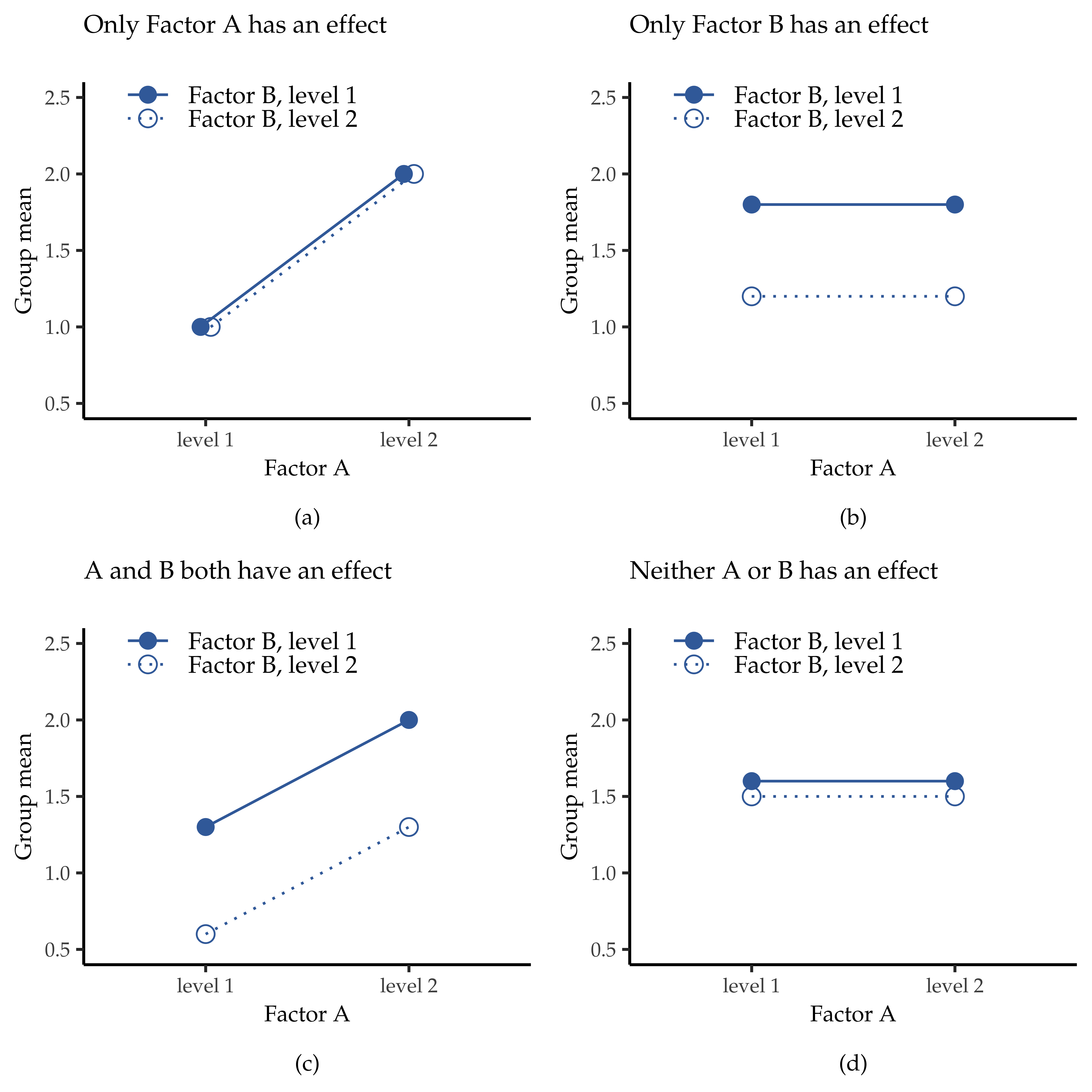
figur 169 The four different outcomes for a 2 × 2 ANOVA when no interactions are present. In the top-left panel, we see a main effect of factor A and no effect of factor B. The top-right panel shows a main effect of factor B but no effect of factor A. The bottom-left panel shows main effects of both factor A and factor B. Finally, the bottom-right panel shows if neither factor has an effect.

What kinds of outcomes does this analysis capture?

The ANOVA model that we have been talking about so far covers a range of different patterns that we might observe in our data. For instance, in a two-way ANOVA design there are four possibilities. An example of each of these four possibilities is plotted in figur 169: (1) only factor A matters (top-left), (2) only factor B matters (top-right), (3) both A and B matter (bottom-left), and (4) neither A nor B matters (bottom-right).

---

[1]

The nice thing about the subscript notation is that it generalises nicely. If our experiment had involved a third factor, then we could just add a third subscript. In principle, the notation extends to as many factors as you might care to include, but in this book we will rarely consider analyses involving more than two factors, and never more than three.

[2]

Technically, marginalising is not quite identical to a regular mean. It is a weighted average where you take into account the frequency of the different events that you are averaging over. However, in a balanced design, all of our cell frequencies are equal by definition so the two are equivalent. We will discuss unbalanced designs later, and when we do so you will see that all of our calculations become a real headache. But let us ignore this for now.

[3]

To put it bluntly: “least tedious”.