Afsnitsforfatter: Danielle J. Navarro and David R. Foxcroft
The Fisher exact test
What should you do if your cell counts are too small, but you would still like
to test the null hypothesis that the two variables are independent? One answer
would be “collect more data”, but that is far too glib. There are a lot of
situations in which it would be either infeasible or unethical do that. If so,
statisticians have a kind of moral obligation to provide scientists with better
tests. In this instance, Fisher (1922a) kindly provided
the right answer to the question. To illustrate the basic idea let us suppose
that we are analysing data from a field experiment looking at the emotional
status of people who have been accused of Witchcraft, some of whom are currently
being burned at the stake.[1] Unfortunately for the scientist (but rather
fortunately for the general populace), it is actually quite hard to find people
in the process of being set on fire, so the cell counts are awfully small in
some cases. A contingency table of the salem data set illustrates the point:
Happy |
Sad |
|
|---|---|---|
Set on fire |
0 |
3 |
Not set on fire |
10 |
3 |
Looking at this data, you would be hard pressed not to suspect that people not on fire are more likely to be happy than people on fire. However, the χ²-test makes this very hard to test because of the small sample size. So, speaking as someone who does not want to be set on fire, I really would like to be able to get a better answer than this. This is where Fisher’s exact test (Fisher, 1922a) comes in very handy.
The Fisher exact test works somewhat differently to the χ²-test (or in fact any of the other hypothesis tests that I talk about in this book) insofar as it does not have a test statistic, but it calculates the p-value “directly”. I will explain the basics of how the test works for a 2 × 2 contingency table. As before, let us have some notation:
Happy |
Sad |
Total |
|
|---|---|---|---|
Set on fire |
O11 |
O12 |
R1 |
Not set on fire |
O21 |
O22 |
R2 |
Total |
C1 |
C2 |
N |
In order to construct the test Fisher treats both the row and column totals (R1, R2, C1 and C2) as known, fixed quantities and then calculates the probability that we would have obtained the observed frequencies that we did (O11, O12, O21 and O22) given those totals. In the notation that we developed in chapter Introduction to probability this is written:
As you might imagine, it is a slightly tricky exercise to figure out what this probability is. But it turns out that this probability is described by a distribution known as the hypergeometric distribution. What we have to do to calculate our p-value is calculate the probability of observing this particular table or a table that is “more extreme”.[2] Back in the 1920s, computing this sum was daunting even in the simplest of situations, but these days it is pretty easy as long as the tables are not too big and the sample size is not too large. The conceptually tricky issue is to figure out what it means to say that one contingency table is more “extreme” than another. The easiest solution is to say that the table with the lowest probability is the most extreme. This then gives us the p-value.
You can specify this test in jamovi from a check box in the Statistics
options of the Contingency Tables analysis. When you do this with the
salem data set, the Fisher's exact test statistic is shown in the
results. The main thing we are interested in here is the p-value, which in
this case is small enough (p = 0.036) to justify rejecting the null
hypothesis that people on fire are just as happy as people not on fire (see
figur 94).
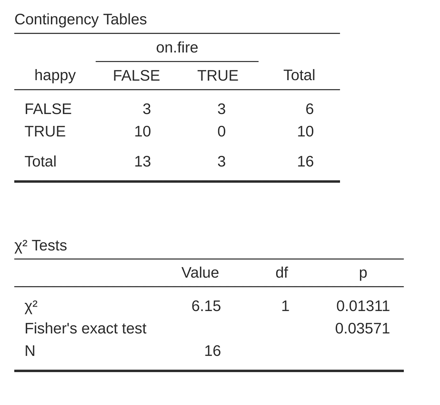
figur 94 Fisher's exact test output in jamovi